Mathematical Modeling of the Self-Compacting Concrete Samples Behavior Produced from The Syrian Raw Materials
2023-04-18 | Volume 1 Issue 1 - Volume 1 | Research Articles | Ammar Tawashi | Soleman Al-AmoudiAbstract
The main purpose of the research is to find a mathematical model describing the behaviour of self-compacting concrete SCC produced from local raw materials only by using mathematical analysis and experimental test results. Three mixtures of SCC were produced: the mixtures with a cement quantity of (550 kg/m3) had been shown satisfying results in the fresh and hardened states and an increase in compression strength up to (12%) and a decrease in the W/C ratio to (13%) compared to the reference samples. The stress-strain (σ,ε) curve was measured for them and compared with the reference curves. The results showed incomplete similarity and the convergence of the curves reaching up to (80%). The closest curve that describes the case is the “POPOVICS” curve with its ascending part and the European Code “EURO-CEB” curve with its descending part. To avoid the presence of two completely different mathematical equations describing the (σ,ε) curves for the SCC made of local materials, a mathematical equation was derived that has one general form, for the two parts of the ascending-descending curve. A direct mathematical calculation and find (σ,ε) curve has been done which accurately describes the behavior of the SCC whatever the quantity of cement.
The list of abbreviations :
(SCC) Self-Compacting Concrete
(σ-ε) The Stress- Strain in Concrete
(SF) Slump Flow
(DJ) J-Ring Test
(VSI) Visual Stability Index
(SR) Segregation Test
(HRW) High Reduction Water
(W/C) Water/Cement Ratio
Keywords : Self-Compacting Concrete, Stress-Strain, Euro-CEB, Popovics, Mathematical Formula.Introduction
Many researchers are concerned with studying the behavior of concrete under the influence of compression loads. Then giving proposals for mathematical models through a mathematical extrapolation that explains the material behavior, which is determined by the relation between stress and strain (σ,ε). However, most of the proposed mathematical equations depend mainly on the results of the experimental tests which could be similar in the general shape with variation in the terms of its application, while depending on the mechanical, chemical, and physical properties of the various particles of concrete. In comparison with the studies that were carried out on concrete containing chemical and filler additives, such as hydraulic, pozzolanic materials, and chemical additives such as plasticizers [1], the topic of SCC self-compacting concrete containing improved materials and the effect of these materials on the molecular structure of the material is considered an important one for research. This is due to the effectiveness and wide spread of this type of modern concrete SCC in many engineering applications. Mohammed H M presented an experimental investigation on the stress-strain behavior of normal [2] and high-strength self-compacting concrete, with two different maximum aggregate sizes. The results show that the ascending parts of the stress-strain curves become steeper as the compressive strength increases, and maximum aggregate size decreases. Jianjie Yu studied the changing regularity of rubber particles’ impact on self-compacting concrete deformation performance [3]. The results show that the rubber particles in self-compacting concrete is more uniform distribution, compared with the reference group. In addition, Selvi K presented an experimental investigation on the modulus of elasticity of self-compacting concrete, involving various flying ash proportions [4], where the stress-strain relationship was studied for the M20 concrete mix. All previous research has studied self-compacting concrete containing fine filler additives, such as flying ash [5]. That gives the concrete distinctive fresh and hardened properties.
This paper will present the production of self-compacting concrete SCC clear of fine fillers by using cement as a fine material that is available and representative of those additives’ fillers.
Materials and Methods
Many previous studies and research have discussed the performance of concrete and described its behavior using the stress-strain curves (σ,ε). This expresses the mechanical behavior of the material [6], throughout deducing a formula that enables us to analyze the behavior of concrete mathematically. In 1951, HOGNESTAD proposed mathematical formula (equations 1 and 2), this enables us to describe the relationship between stress and strain in the ascending, and descending parts of curves [7] for traditional concrete. Figure /1/. So, stress f_c is calculated as a function of the relative strain $ (\frac{\varepsilon_c}{\varepsilon_{co}}) $.
$ f_{c,1}=0.85{f\prime}_c\left[2\frac{\varepsilon_c}{\varepsilon_{co}}-{(\frac{\varepsilon_c}{\varepsilon_{co}})}^2\right]\ \ \ \ \ \ \ \ \ \ \ \ \ \ \ \ \ \ \ \ \ \ \ \ 0>\varepsilon_c>\varepsilon_{co} $ (1)
$ f_{c,2}=0.85{f\prime}_c\left[1-{0.15(\frac{\varepsilon_c-\varepsilon_{co}}{\varepsilon_{cu}-\varepsilon_{co}})}^2\right]\ \ \ \ \ \ \ \ \ \ \ \ \varepsilon_{co}>\varepsilon_c>\varepsilon_{cu} $ (2)
$ f_{c,1} $: the stress of the concrete in the ascending part MPa.
$ f_{c,2} $: the stress of the concrete in the descending part MPa.
$ {f\prime}_c $: the maximum compression strength of the concrete MPa.
$ \varepsilon_{co} $: the strain corresponding to the maximum compression strength of the concrete.
$ \varepsilon_{cu} $: the critical strain of the concrete.
$ \varepsilon_c $: the strain of the concrete.
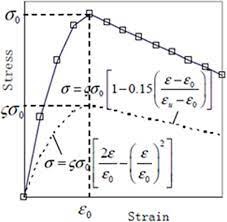
Fig. 1. HOGNESTAD stress-strain curve
KENT and PARK also presented, in 1971, a proposal for a stress-strain curve model Equation 3 for the confined and unconfined concrete with the descending part only [8]. Figure /2/. So, the stress fc is calculated as a function of the strain corresponding to the maximum strain εco, and the critical strain
$ f_c={f\prime}_c\left[1-\frac{0.5}{\varepsilon_{50u}-\varepsilon_{co}}(\varepsilon_c-\varepsilon_{co})\right]\ \ \ \ \ \ \ \ \ \ \ \ \ \varepsilon_{co}>\varepsilon_c>\varepsilon_{cu} $ (3)
$ \varepsilon_{50u}=\frac{3+0.29{f^\prime}_c}{145{f^\prime}_c-1000}{f^\prime}_c(Mpa) $

Fig. 2. KENT and PARK stress-strain curve
Also, in 1973 POPOVICS presented mathematical formulas. Equation /4/ describing the stress-strain relation of concrete [9]. It was considered that the relative stress as a function of the relative strain according to the following:
$ \frac{f_c}{{f\prime}_c}=\left[\frac{n\frac{\varepsilon_c}{\varepsilon_{co}}}{\left(n-1\right)+{(\frac{\varepsilon_c}{\varepsilon_{co}})}^n}\right] $ (4)
$ n=0.058.{f\prime}_c+1 $
He also presented a mathematical formula. Equation 5. in order to calculate the strain of concrete as a function of the maximum compression strength in the concrete:
$ \varepsilon_{co}=\frac{2{f\prime}_c}{12500+450{f\prime}_c} $ (5)
As for CARREIRA, he followed what POPOVICS had reached and developed a mathematical formula. Equation /6/ for calculating stress as a function of strain [3], where he took the effect of the concrete elasticity factor into account. As follows:
$ \frac{f_c}{{f\prime}_c}=\left[\frac{R(\frac{\varepsilon_c}{\varepsilon_{co}})}{\left(R-1\right)+{(\frac{\varepsilon_c}{\varepsilon_{co}})}^R}\right] $ (6)
$ R=\frac{E_c}{E_c-E_O} $
Where:
$ E_c=5000.\sqrt{{f\prime}_c}\ Mpa $
$ E_O=\frac{{f\prime}_c}{\varepsilon_{co}} $
$ ???: is the strain at the maximum compressive strength of confined concrete ?′?. $
The European Code EN 1992-1-1 also presented a mathematical formula. Equation /7/describes the stress-strain behavior of concrete [4] as a function of the relative strain $ \frac{\varepsilon_c}{\varepsilon_{co}}, $, and related to the elasticity factor of the material. According to the following:
$ \frac{f_c}{{f\prime}_c}=\left[\frac{k\eta-\eta^2}{1+(k-2)\eta}\right] $
$ \eta=\frac{\varepsilon_c}{\varepsilon_{co}} $
$ k={1.05.E}_c\frac{\varepsilon_{co}}{{f\prime}_c} $
SCOPE OF WORK
The Fresh Properties of Self-Compacting Concrete
Three mixtures of self-compacting concrete SCC were produced, in addition to the reference mixture, in different cement quantities [11]. The proportions of materials for the mixes are given in Table 1.
Table 1. The proportions of materials
| Mixture | Cement quantity (kg/m3) | W/C | Superplasticizer (%) | Coarse Aggregates (kg/m3) | Fine Aggregates (kg/m3) |
| SCC | 550
500 450 |
0.390 | 2.0
2.5 2.5 |
625 | 1000 |
The tests of the fresh properties of SCC were conducted [14]. They include J-ring Test, Slump Flow (SF) and Test, Visual Stability Index (VSI), and Segregation Test (SR). As shown in Figure 3.
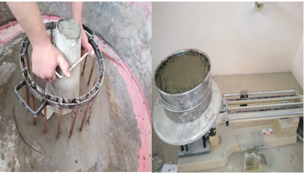
Fig. 3. SCC-HRW Fresh Properties Tests
The rules for adopting the ratio of superplasticizer depend on the technical specification and guidelines for using this type of material, where the recommended ratio range (from 0.5 to 2.5) % of cement weight. In the lab tests, the initial ratio was 1% and then increased till it achieved the required operability in each one of the mixes.
It was found that the mixture with a proportion of cement quantity (550 kg/m3) containing plasticizer coded as HRW gives the preferred properties the operability, Table /2/. The mixture with (450 kg/m3) cement quantity does not give any of the required properties for this type of concrete.
Table 2. SCC fresh properties:
| Mixture | Cement quantity (kg/m3) | W/C | Superplasticizer (%) | Slump Flow SF (cm) | (sec) | J-ring (DJ %) | Segregation Test (SR%) | |
| SCC-HRW-550 | 550 | 0.39 | 2.0 | 58 | 5.40 | 86 | 6.42 | |
| SCC-HRW-500 | 500 | 0.39 | 2.5 | 52 | 4.86 | 96 | 4.06 | |
| SCC-HRW-450 | 450 | 0.39 | 2.5 | – | – | – | – | |
| Allowed | 55-65 | – | ≥80% | ≤15% | ||||
Strength of SCC Samples on the Axial Compression
The laboratory tests result of SCC cylindrical samples produced locally at uni-axial compression [13] show the contribution of the plasticizer by reducing the ratio W/C up to 13%. Thus, there is an improvement in the SCC concrete in terms of strength and strain behavior. Figure 4.
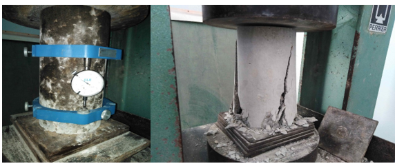
Fig. 4. Fracture Test of SCC Cylindrical Samples
According to laboratory tests, an increase in the strength of concrete containing plasticizer HRW (high reduction water) by 2% of the cement weight up to 12% has been noted, compared to the reference sample, which has the same proportions of materials but without a plasticizer.
The plasticizer in all concrete mixtures contributed to an increase in the operability and a decrease in the W/C ratio. The percentage up in the strength was due to the quantity of cement used, the type of plasticizer, the percentage of plasticizer, and the W/C ratio [12]. The decrease in the compression strength was observed by using a lower quantity of cement with a higher percentage of plasticizer. This can be explained by the change in the molecular structure of SCC mixtures when the ratio W/C is stable. So, it is better to use a higher quantity of cement for a lower plasticizer percentage, and stability by a ratio of W/C.
Since the concrete molecular structure is made up of two components, aggregates and paste. Aggregates are generally classified into two groups, fine and coarse, and occupy about 70% of the mix volume. The paste is composed of cement, water, and entrained air and ordinarily constitutes 30% of the remaining volume.
The major change in the molecular structure of the mixture under the influence of the superplasticizer is on the cement paste, which affects one component or more of the three mentioned.
Table 3. below shows the increase in the cylindrical compression strength depending on the cement quantity, the percentage of plasticizer, and W/C ratio.
Table 3. Compressive strength of SCC mixtures
| Mixture | Cement quantity (kg/m3) | W/C | Superplasticizer (%) | Compression Strength (MPa) | Strength Increase Ratio (%) |
| RS-550 | 550 | 0.448 | – | 33,572 | – |
| SCC-HRW-550 | 550 | 0.39 | 2 | 37.616 | 12 |
| RS-500 | 500 | 0.448 | – | 27.717 | – |
| SCC-HRW-500 | 500 | 0.39 | 2.5 | 28.249 | 1.9 |
| RS-450 | 450 | 0.448 | – | 24.680 | – |
| SCC-HRW-450 | 450 | 0.39 | 2.5 | 24.890 | 0.01 |
In the mixes with cement quantities 450 kg/m3, it is noted that the compression strength takes the same result with or without a plasticizer. This can explain the excess dose of the plasticizer causes additional dispersion and scattering of the cement granules, due to the repulsion of the negative charges that envelop them. Thus, there was a lack of bonding of the cement granules. Another reason that could occur was an increase in the additional air to the mixture.
Figure 5. shows the relation between the strength and the plasticizer percentage used, according to the quantity of cement in the SCC samples.

Fig. 5. SCC Strength and Plasticizer Percentage Relation
According to the previous data of the tests, and by searching for the mathematical equation that is closest and most representative of the relation between the strength of SCC and cement quantity and by using Curve Expert1.4 software program for processing curves, many mathematical curves were obtained. Figure 6. shows the closest curves to the study case with correlation coefficient R.
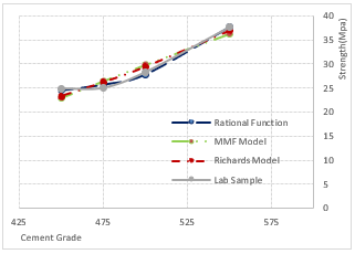
Fig. 6. The Closest Mathematical Curves
The above three mathematical graphic curves are closest to our experimental tests. It is clear from Figure 6 that the model known as the Rational Function gives the closest model with the best correlation factor R closer to 1. Equation 8, the realistic behaviour of the SCC, and the most expressive of the relation between the cement quantity and the strength of the self-compacting concrete, on the axial compression for different plasticizer ratios. While the other curves show a continuous sharp decline in the strength between the defined points, and an infinitely increasing of strength. This contradicts the relation between the concrete strength and the cement grade.
The Equation of Rational Function is given as:
$ y=\frac{a+bx}{1+cx+dx^2} $ (8)
y: Compression Strength of SCC (MPa).
x: Cement Grade (kg/m3).
a,b,c,: Equation constants, substituting the values of the constants into Equation (1). Founded that the equation takes the following form (9):
$ y=\frac{-45572.93+48.36x}{1-7.74x+0.0124x^2} $
Proposed Model of the Stress-Strain Formula for the Self-Compacting Concrete
The chemical materials in the self-compacting concrete led to a change in the molecular composition of the material. Thus, a change in its mechanical properties affects the behaviour of the concrete in fresh and hardened cases.
Through the application and analysis of previous models of the relation between stress-strain on SCC prepared in the lab, it was found that models can express the behaviour of concrete SCC in varying proportions. As for, the convergence was clear with the lab model, in the ascending part of the curve until reaching the ultimate stress Figure 7. But the difference was in the descending part of the curve. Therefore, it was interesting to search for a mathematical model that describing and expressing the closest behaviour for SCC in ascending and descending parts of the curve.
To understand the behaviour of hardened concrete, and through accurate processing of the numerical results of the fracture tests on the uni-axial compression of cylindrical samples. Models were achieved to describe the stress-strain occurred under the influence of the uni-axial compressive force.
To obtain a general unconditional formula, unrestricted in terms of the quantity of cement and the proportion of plasticizer used in the mixture. Data were processed and converted into non-dimensional relative values allowing the conversion of the data from the specific case into the general state of the tested concrete.
 Fig. 7. SCC and Reference Stress-Strain Curves
It was started from the same premise of previous studies and models in mathematical treatment by converting stress f_c into relative stress by dividing it by $ {f\prime}_c $, and the measured strain \varepsilon_c into relative strain by dividing it by $ \varepsilon_{co} $. So, the values of the mathematical treatment for stress and strain, are according to the following:
$ \frac{f_c}{{f\prime}_c} $: nominal relative stress, where: $ {f\prime}_c $: the maximum cylindrical strength of the concrete.
$ \frac{\varepsilon_c}{\varepsilon_{co}} $: nominal relative strain, where:$ \varepsilon_{co} $: strain corresponding to the maximum stress of the concrete.
To find a mathematical model that expresses the behavior of this type of concrete, the results of lab experiments of samples produced of SCC were entered at several cement quantities, and by defining it as nominal relative values $ \frac{f_c}{{f\prime}_c} $, $ \frac{\varepsilon_c}{\varepsilon_{co}} $ to obtain the optimal mathematical curve for this case, which gives the best correlation coefficient R and the smallest standard error.
The treatment showed that the most appropriate mathematical formula for the curve, in this case, is the Rational Function form, Equation 10. which is the general form:
$ y=\frac{a+bx}{1+cx+dx^2} $ (10)
y: the compressive strength in the concrete.
x: the strain in the concrete.
a, b, c, d equation constants.
The equation shown above and in its general form does not achieve the conditions of the model we are looking for, in terms of stress and relative strain. Figure 8 below shows the experimental and the equation curves form:
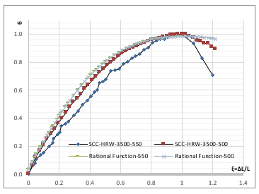
Fig. 8. SCC and Rational Function Equation Stress-Strain Curves
Starting from the performance form of the SCC expressed by the stress-strain curve. The equation was reformulated of the closed model in its general form, using the values of relative stress and strain. So that form of Equation 11. and Equation 12. becomes according to the following:
$ \frac{f_c}{{f\prime}_c}=\frac{a+b(\frac{\varepsilon_c}{\varepsilon_{co}})}{1+c(\frac{\varepsilon_c}{\varepsilon_{co}})+d{(\frac{\varepsilon_c}{\varepsilon_{co}})}^2} $ (11)
$ f_{cnorm}=\frac{a+b(\varepsilon_{cnorm})}{1+c(\varepsilon_{cnorm})+d{(\varepsilon_{cnorm})}^2} $ (12)
$ f_{cnorm}=\frac{f_c}{{f\prime}_c} $ nominal relative stress
$ \varepsilon_{cnorm}=\frac{\varepsilon_c}{\varepsilon_{co}} $ nominal relative strain.
 Therefore, the proposed general mathematical formula could be expressed with the values of constant b in the ascending and descending parts of the curve.
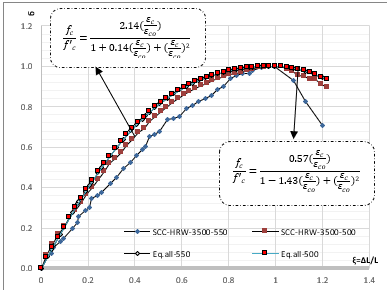 Fig. 9. Stress-Strain Curves for SCC and Proposed Eq. at all Cement Grade
$ \frac{f_c}{{f\prime}_c}=\left[\frac{n\frac{\varepsilon_c}{\varepsilon_{co}}}{\left(n-1\right)+{(\frac{\varepsilon_c}{\varepsilon_{co}})}^n}\right] $ (20)
Through the observation of the two formulas, there is an incomplete similarity in general. However. this similarity can be complete when the value of the constants as below:
n=b=2
The proposed and POPOVICS formulas take the following form 21:
$ \frac{f_c}{{f\prime}_c}=\frac{2\frac{\varepsilon_c}{\varepsilon_{co}}}{1+{(\frac{\varepsilon_c}{\varepsilon_{co}})}^2} $ (21)
It can also verify the conformity of the behaviour proposed in Eq.21 with the actual samples graphically. Below are the stress-strain curves of the proposed formula and the experimental sample. Figure .10:
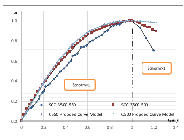
Fig. 10. Stress-Strain Curves for The SCC Proposed Mathematical Formula
It has been found that the mathematical equation 21 in which the POPOVICS formula and the proposed formula are similar, gives graphic curves describing the behavior of local SCC with a convergence of up to 90%.
CONCLUSION
This paper aimed to understand the mechanical behavior of SCC samples. Through laboratory verification and mathematical analysis. The key findings of this study are presented below:
The possibility to produce an acceptable Self-Compacting Concrete SCC from Syrian raw materials.
Outputting a mathematical model that enables us to directly calculate the behavior of all types of SCC samples, and to represent it graphically.
The proposed mathematical model describes the behavior of concrete up to 90% approximate, whatever the quantity of cement.
References :- American Society for Testing and Materials, ASTM. Standard Specification for Chemical Admixtures for Concrete. C 494 – 03. Annual Book of ASTM Standard. United States; 2003. Vol: 04.02.
- Mohammed H M. Stress-strain behavior of normal and high strength self-compacting concrete. Materials Science and Engineering. 2020; 737:1-9.
- Jianjie Yu. Research on the Mechanical Properties of Self-compacting Waste Rubberised Aggregate Concrete. International Conference on Civil: Transportation and Environment ICCTE; 2016. p. 88-92.
- Salvi K, Mahendran T, Atthikumaran N. Experimental Investigation on Modulus of Elasticity of Self-Compacting Concrete. Journal of Applied Physics and Engineering (JAPE). 2016; 1(2): 5-8.
- BIBM, CEMBUREAU, EFCA, EFNARC, ERMCO. The European Guidelines for Self-Compacting Concrete Specification, Production and Use. SCC European Project Group SCC 028 European Federations; 2005. p.1-63.
- Wang P T, Shah S P, Naaman A E. Stress-Strain Curve of Normal and Lightweight Concrete in Compression. ACI Journal. 1978; 75(11): 603-611.
- Hognestad E. A study on combined bending and axial load in reinforced concrete members. United State: University of Illinois Engineering Experiment Station Bulletin Series; 1951.
- Kent DC, Park R. Flexural members with confined concrete. Journal of the Structural Division. 1971; 97(ST7): 1969-1990.
- BIBM, CEMBUREAU, EFCA, EFNARC, ERMCO. The European Guidelines for Self-Compacting Concrete Specification, Production and Use. SCC European Project Group SCC 028 European Federations; 2005. p.1-63.
- Carreira DJ, Chu KH. Stress-Strain Relationship for plain concrete in compression. Journal of the American Concrete Institute. 1985; 82(6):797-804.
- Eurocode 2. Design of concrete structures-Part 1-1: General rules and rules for buildings. Ref. No. EN 1992-1-1. The European Union. Belgium; 2004. E 227: p. 27-37.
- TIMO W. Fresh Properties of Self-Compacting Concrete (SCC). Otto – Graf Journal. 2003; 14(10): 179-188.
- Tawashi A, Alamoudi S. The Mechanical Behavior of Self-Compacting Concrete SCC Samples Locally Produce. Journal of Engineering Sciences and Information Technology (AJSRP). 2022; 6(2): 148-169.
- The Syrian Arab Code. The design and implementation the construction by reinforced concrete. Syrian Engineers Association. Fourth Edition. Damascus; 2012. 402: p. 57-69 (In Arabic).
- Tawashi A, Alamoudi S. Study of Stress-Strain behavior of self-compacting concrete SCC Cylindrical Samples Produced of Local Materials. Journal of AL Baath University. 2022; 44(5): 51-74.
The authors declare that they have no competing interests.
Data and materials availability:
All data are available in the main text or the supplementary materials.
(ISSN - Online)
2959-8591