INTRODUCTION
Nowcasting refers to the projection of information about the present, the near future, and even the recent past. The importance of nowcasting has shifted from weather forecasting to economics, where economists use it to track the economy status through real-time GDP forecasts, as it is the main low-frequency (quarterly – annually) indicator reflecting the state of the country’s economy. This is like satellites that reflect the weather on earth. It does this by relying on high-frequency measured variables (daily – monthly) that are reported in real-time. The importance of using nowcasting in the economy stems from the fact that data issuers, statistical offices and central banks release the main variables of the economy, such as gross domestic product and its components, with a long lag. In some countries, it may take up to five months. In other countries, it may take two years depending on the capabilities each country has, leading to a state of uncertainty about the economic situation among economic policy makers and state followers business. Real-time indicators related to the economy (e.g consumer prices and exchange rates) are used here in order to obtain timely information about variables published with a delay. The first use of nowcasting technology in economics dates back to Giannone et al 2008, by developing a formal forecasting model that addresses some of the key issues that arise when using a large number of data series released at varying times and with varying delays [1]. They combine the idea of “bridging” the monthly information with the nowcast of quarterly GDP and the idea of using a large number of data releases in a single statistical framework. Banbura et al proposed a statistical model that produces a series of Nowcasting forecasts on real-time releases of various economic data [2]. The methodology enables the processing of a large amount of information from nowcasting’s Eurozone GDP Q4 2008 study. Since that time, the models that can be used to create nowcasting have expanded. Kuzin et al compared the mixed-frequency data sampling (MIDAS) approach proposed by Ghysels et al [4,5] with the mixed-frequency VAR (MF-VAR) proposed by Zadrozny and Mittnik et al [6,7], with model specification in the presence of mixed-frequency data in a policy-making situation, i.e. nowcasting and forecasting quarterly GDP growth in Eurozone on a monthly basis. After that time, many econometric models were developed to allow the use of nowcasting and solve many data problems. Ferrara et al [8] proposed an innovative approach using nonparametric methods, based on nearest neighbor’s approaches and on radial basis function, to forecast the monthly variables involved in the parametric modeling of GDP using bridge equations. Schumacher et al [9] compare two approaches from nowcasting GDP: Mixed Data Sampling (MIDAS) regressions and bridge equations. Macroeconomics relies on increasingly non-standard data extracted using machine learning (text analysis) methods, with the analysis covering hundreds of time series. Some studies examined US GDP growth forecasts using standard high-frequency time series and non-standard data generated by text analysis of financial press articles and proposed a systematic approach to high-dimensional time regression problems [10-11]. Another team of researchers worked on dynamic factor analysis models for nowcasting GDP [12], using a Dynamic Factor Model (DFM) to forecast Canadian GDP in real-time. The model was estimated using a mix of soft and hard indices and the authors showed that the dynamic factor model outperformed univariate criteria as well as other commonly used nowcasting models such as MIDAS and bridge regressions. Anesti et al [13] proposed a release-enhanced dynamic factor model (RA-DFM) that allowed quantifying the role of a country’s data flow in the nowcasting of both early (GDP) releases and later revisions of official estimates. A new mixed-frequency dynamic factor model with time-varying parameters and random fluctuations was also designed for macroeconomic nowcasting, and a fast estimation algorithm was developed [14]. Deep learning models also entered the field of GDP nowcasting, as in many previous reports [15-17]. In Syria, there are very few attempts to nowcasting GDP, among which we mention a recent report that uses the MIDAS Almon Polynomial Weighting model to nowcasting Syria’s annual GDP based on the monthly inflation rate data [18]. Our research aims to solve a problem that exists in the Arab and developing countries in general, and Syria in particular, namely the inability to collect data in real-time on the main variable in the economy due to the weakness of material and technical skills. Therefore, this study uses Bayesian mixed-frequency VAR models to nowcast GDP in Syria based on a set of high-frequency data. The rationale for choosing these models is that they enable the research goal to be achieved within a structural economic framework that reduces statistical uncertainty in the domain of high-dimensional data in a way that distinguishes them from the nowcasting family of models, according to a work by Cimadomo et al and Crump et al [19-20]. The first section of this research includes the introduction and an overview of the previous literature. The second section contains the research econometric framework, through which the architecture of the research model is developed within a mathematical framework. The third section is represented by the data used in the research including the exploratory phase. The fourth section contains the discussion and interpretation of the results of the model after the evaluation. The fifth section presents the results of the research and proposals that can consider a realistic application by the authorities concerned.
MATERIALS AND METHODS
The working methodology in this research is divided into two main parts. The first in which the low-frequency variable (Gross Domestic Product) is converted from annual to quarterly with the aim of reducing the forecast gap and tracking the changes in the GDP in Syria in more real-time., by reducing the gap with high-frequency data that we want to predict their usage. To achieve this, we used Chow-Lin’s Litterman: random walk variant method.
Chow-Lin’s Litterman Method
This method is a mix and optimization of two methods. The Chow-Lin method is a regression-based interpolation technique that finds values of a series by relating one or more higher-frequency indicator series to a lower-frequency benchmark series via the equation:
x(t)=βZ(t)+a(t) (1)
Where is a vector of coefficients and a random variable with mean zero and covariance matrix Chow and Lin [21] used generalized least squares to estimate the covariance matrix, assuming that the errors follow an AR (1) process, from a state space model solver with the following time series model:
a(t)=ρa(t-1)+ϵ(t) (2)
Where ϵ(t)~N(0,σ^2) and |ρ|<1. The parameters ρ and βare estimated using maximum likelihood and Kalman filters, and the interpolated series is then calculated using Kalman smoothing. In the Chow-Lin method, the calculation of the interpolated series requires knowledge of the covariance matrix, which is usually not known. Different techniques use different assumptions about the structure beyond the simplest (and most unrealistic) case of homoscedastic uncorrelated residuals. A common variant of Chow Lin is Litterman interpolation [22], in which the covariance matrix is computed from the following residuals:
a(t)=a(t-1)+ϵ(t) (3)
Where ϵ(t)~N(0,V)
ϵ(t)=ρϵ(t-1)+e(t) (4)
and the initial state a(0)=0. . This is essentially an ARIMA (1,1,0) model.
In the second part, an econometric model suitable for this study is constructed by imposing constraints on the theoretical VAR model to address a number of statistical issues related to the model’s estimation, represented by the curse of dimensions.
Curse of Dimensions
The dimensional curse basically means that the error increases with the number of features (variables). A higher number of dimensions theoretically allows more information to be stored, but rarely helps as there is greater potential for noise and redundancy in real data. Collecting a large number of data can lead to a dimensioning problem where very noisy dimensions can be obtained with less information and without much benefit due to the large data [23]. The explosive nature of spatial scale is at the forefront of the Curse of Dimensions cause. The difficulty of analyzing high-dimensional data arises from the combination of two effects: 1- Data analysis tools are often designed with known properties and examples in low-dimensional spaces in mind, and data analysis tools are usually best represented in two- or three-dimensional spaces. The difficulty is that these tools are also used when the data is larger and more complex, and therefore there is a possibility of losing the intuition of the tool’s behavior and thus making wrong conclusions. 2- The curse of dimensionality occurs when complexity increases rapidly and is caused by the increasing number of possible combinations of inputs. That is, the number of unknowns (parameters) is higher than the number of observations. Assuming that m denotes dimension, the corresponding covariance matrix has m (m+1)/2 degrees of freedom, which is a quadratic term in m that leads to a high dimensionality problem. Accordingly, by imposing a skeletal structure through the initial information of the Bayesian analysis, we aimed to reduce the dimensions and transform the high-dimensional variables into variables with lower dimensions and without changing the specific information of the variables. With this, the dimensions were reduced in order to reduce the feature space considering a number of key features.
Over Parameterizations
This problem, which is an integral part of a high dimensionality problem, is statistically defined as adding redundant parameters and the effect is an estimate of a single, irreversible singular matrix [24]. This problem is critical for statistical estimation and calibration methods that require matrix inversion. When the model starts fitting the noise to the data and the estimation parameters, i.e. H. a high degree of correlation existed in the co-correlation matrix of the residuals, thus producing predictions with large out-of-sample errors. In other words, the uncertainty in the estimates of the parameters and errors increases and becomes uninterpretable or far from removed from the realistic estimate. This problem is addressed by imposing a skeletal structure on the model, thereby transforming it into a thrift. Hence, it imposes constraints that allow a correct economic interpretation of the variables, reducing the number of unknown parameters of the structural model, and causing a modification of the co – correlation matrix of the residuals so that they become uncorrelated with some of them, in other words, become a diagonal matrix.
Overfitting and Underfitting
Overfitting and Underfitting are major contributors to poor performance in models. When Overfitting the model (which works perfectly on the training set while ineffectively fitting on the test set), it begins with matching the noise to the estimation data and parameters, producing predictions with large out-of-sample errors that adversely affect the model’s ability to generalize. An overfit model shows low bias and high variance [25]. Underfitting refers to the model’s inability to capture all data features and characteristics, resulting in poor performance on the training data and the inability to generalize the model results [26]. To avoid and detect overfitting and underfitting, we tested the validity of the data by training the model on 80% of the data subset and testing the other 20% on the set of performance indicators.
Theoretical VAR model
VAR model developed by Sims [27] has become an essential element in empirical macroeconomic research. Autoregressive models are used as tools to study economic shocks because they are based on the concept of dynamic behavior between different lag values for all variables in the model, and these models are considered to be generalizations of autoregressive (AR) models. The p-rank VAR is called the VARp model and can be expressed as:
y_t=C+β_1 y_(t-1)+⋯+β_P y_(t-P)+ϵ_t ϵ_t~(0,Σ) (5)
Where y_t is a K×1 vector of endogenous variables. Is a matrix of coefficients corresponding to a finite lag in, y_t, ϵ_t: random error term with mean 0 representing external shocks, Σ: matrix (variance–covariance). The number of parameters to be estimated is K+K^2 p, which increases quadratic with the number of variables to be included and linearly in order of lag. These dense parameters often lead to inaccuracies regarding out-of-sample prediction, and structural inference, especially for high-dimensional models.
Bayesian Inference for VAR model
The Bayesian approach to estimate VAR model addresses these issues by imposing additional structure on the model, the associated prior information, enabling Bayesian inference to solve these issues [28-29], and enabling the estimation of large models [2]. It moves the model parameters towards the parsimony criterion and improves the out-of-sample prediction accuracy [30]. This type of contraction is associated with frequentist regularization approaches [31]. Bayesian analysis allows us to understand a wide range of economic problems by adding prior information in a normal way, with layers of uncertainty that can be explained through hierarchical modelling [32].
Prior Information
The basic premise for starting a Bayesian analysis process must have prior information, and identifying it correctly is very important. Studies that try not to impose prior information result in unacceptable estimates and weak conclusions. Economic theory is a detailed source of prior information, but it lacks many settings, especially in high-dimensional models. For this reason, Villani [33] reformulates the model and places the information at a steady state, which is often the focus of economic theory and which economists better understand. It has been proposed to determine the initial parameters of the model in a data-driven manner, by treating them as additional parameters to be estimated. According to the hierarchical approach, the prior parameters are assigned to hyperpriors. This can be expressed by the following Bayes law: 
Wherey= (y_(p+1)+⋯+y_T)^T,θ: is coefficients AR and variance for VAR model, γ: is hyperparameters. Due to the coupling of the two equations above, the ML of the model can be efficiently calculated as a function of γ. Giannone et al [34] introduced three primary information designs, called the Minnesota Litterman Prior, which serves as the basis, the sum of coefficients [35] and single unit root prior [36].
Minnesota Litterman Prior
Working on Bayesian VAR priors was conducted by researchers at the University of Minnesota and the Federal Reserve Bank of Minneapolis [37] and these early priors are often referred to as Litterman prior or Minnesota Prior. This family of priors is based on assumption that Σ is known; replacing Σwith an estimate Σ. This assumption leads to simplifications in the prior survey and calculation of the posterior.
The prior information basically assumes that the economic variables all follow the random walk process. These specifications lead to good performance in forecasting the economic time series. Often used as a measure of accuracy, it follows the following torques:

The key parameter ⋋ is which controls the magnitude influence of the prior distribution, i.e. it weighs the relative importance of the primary data. When the prior distribution is completely superimposed, and in the case of the estimate of the posterior distributions will approximate the OLS estimates. is used to control the break attenuation, and is used to control the prior standard deviation when lags are used. Prior Minnesota distributions are implemented with the goal of de-emphasizing the deterministic component implied by the estimated VAR models in order to fit them to previous observations. It is a random analysis-based methodology for evaluating systems under non-deterministic (stochastic) scenarios when the analytical solutions are complex, since this method is based on sampling independent variables by generating phantom random numbers.
Dummy Observations
Starting from the idea of Sims and Zha [38] to complement the prior by adding dummy observations to the data matrices to improve the predictive power of Bayesian VAR. These dummy observations consist of two components; the sum-of-coefficient component and the dummy-initial-observation component. The sum-of-coefficients component of a prior was introduced by Doan et al [37] and demonstrates the belief that the average of lagged values of a variable can serve as a good predictor of that variable. It also expresses that knowing the average of lagged values of a second variable does not improve the prediction of the first variable. The prior is constructed by adding additional observations to the top (pre-sample) of the data matrices. Specifically, the following observations are constructed: 
Where is the vector of the means over the first observed by each variable, the key parameter is used to control for variance and hence the impact of prior information. When the prior information becomes uninformative and when the model is formed into a formula consisting of a large number of unit roots as variables and without co-integration. The dummy initial observation component [36] creates a single dummy observation that corresponds to the scaled average of the initial conditions, reflecting the belief that the average of the initial values of a variable is likely to be a good prediction for that variable. The observation is formed as:

Where is the vector of the means over the first observed by each variable, the key parameter is used to control on variance and hence the impact of prior information. As , all endogenous variables in VAR are set to their unconditional mean, the VAR exhibits unit roots without drift, and the observation agrees with co-integration.
Structural Analysis
The nowcasting technique within the VAR model differs from all nowcasting models in the possibility of an economic interpretation of the effect of high-frequency variables on the low-frequency variable by measuring the reflection of nonlinear changes in it, which are defined as (impulse and response). A shock to the variable not only affects the variable directly, but it is also transmitted to all other endogenous variables through the dynamic (lag) structure of VAR. An impulse response function tracks the impact of a one-off shock to one of the innovations on current and future values of the endogenous variable.
BVAR is estimated reductively, i.e., without a contemporary relationship between endogenous variables in the system. While the model summarizes the data, we cannot determine how the variables affect each other because the reduced residuals are not orthogonal. Recovering the structural parameters and determining the precise propagation of the shocks requires constraints that allow a correct economic interpretation of the model, identification constraints that reduce the number of unknown parameters of the structural model, and lead to a modification of the co-correlation matrix of the residuals so that they become uncorrelated, i.e., they become a diagonal matrix. This problem is solved by recursive identification and achieved by Cholesky’s analysis [39] of the variance and covariance matrix of the residuals , Where Cholesky uses the inverse of the Cholesky factor of the residual covariance matrix to orthogonalize the impulses. This option enforces an ordering of the variables in the VAR and attributes the entire effect of any common component to the variable that comes first in the VAR system. For Bayesian frame, Bayesian sampling will use a Gibbs or Metropolis-Hasting sampling algorithm to generate draws from the posterior distributions for the impulse. The solution to this problem can be explained mathematically from the VAR model:
![]()
Where show us contemporaneous correlation. Coefficient matrix at lag1, error term where:

In order to estimate the previous equation, we must abandon the contemporaneous relations between the endogenous variables since we transfer them to the other side:
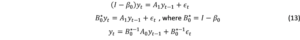
Now parsimony VAR model can be estimated:
![]()
Where A_1 are reduced coefficient. u_t Represent the weighted averages of the structural coefficientsβ_1,ϵ_t. Where:
 Mixed Frequency VAR
Complementing the constraints imposed on the theoretical VAR model, as a prelude to achieving the appropriate form for the research model and developing the model presented by AL-Akkari and Ali [40] to predict macroeconomic data in Syria, we formulate the appropriate mathematical framework for the possibility to benefit from high-frequency data emitted in real-time in nowcasting of GDP in Syria.
We estimate a mixed frequency VAR model with no constant or exogenous variables with only two data frequencies, low and high (quarterly-monthly), and that there are high frequency periods per low frequency period. Our model consists of variable observed at low frequency and variables observed at high frequency. Where:
: represent the low-frequency variable observed during the low-frequency period .
: represent the high-frequency variable observed during the low-frequency period .
By stacking the and variables into the matrices and ignoring the intersections and exogenous variables for brevity, respectively, we can write the VAR:

Performance indicators
We use indicators to assess the performance of the models which are used to determine their ability to explain the characteristics and information contained in the data. It does this by examining how closely the values estimated from the model correspond to the actual values, taking into account the avoidance of an underfitting problem that may arise from the training data and an overfitting problem that arises from the test data. The following performance indicators include:
Theil coefficient (U):
 Mean Absolute Error (MAE):
![]()
Root Mean Square Error (RMSE): 
Where the forecast is value; is the actual value; and is the number of fitted observed. The smaller the values of these indicators, the better the performance of the model.
RESULTS & DISCUSSION
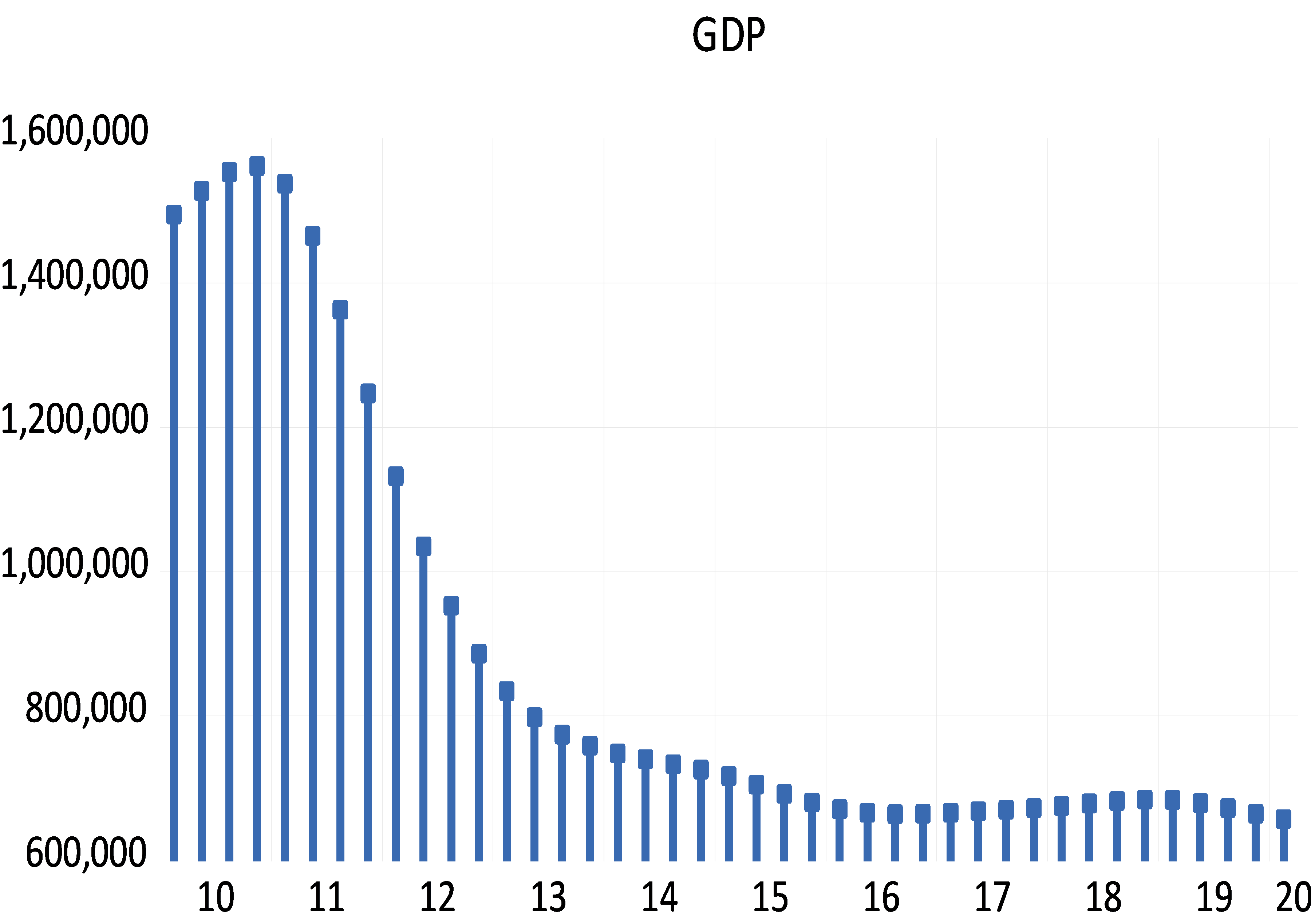
As mentioned, the data consists of high and low frequency variables collected from the websites of official Syrian organizations and the World Bank [41-46], summarized in Table 1, which shows basic information about data. The data of the variable GDP were collected annually and converted using the combination of Chow-Lin’s Litterman methods, (Fig 1), which shows that the volatility in annual GDP was explained by the quarter according to the hybrid method used, and gives us high reliability for the possibility of using this indicator in the model. For high-frequency data, the monthly closing price was collected from the sources listed in Table (1) and its most recent version was included in the model to provide real-time forecasts.

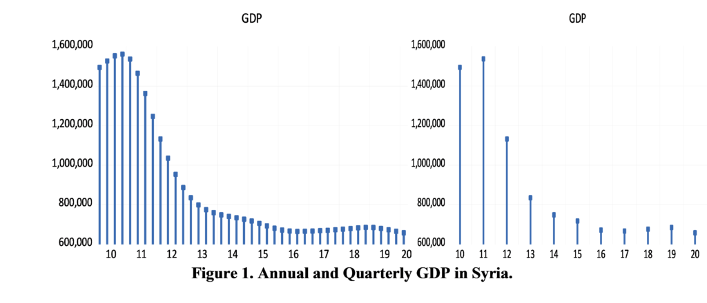
Figure (2) shows the evolution of these variables. We presented in Figure (2), the data in its raw form has a general stochastic trend and differs in its units of measurement. To unify the characteristics of this data, growth rates were used instead of prices in this case, or called log, because of their statistical properties. These features are called stylized facts; first, there is no normal distribution. In most cases, the distribution deviates to the left and has a high kurtosis. It has a high peak and heavy tails [47]. Second, it has the property of stationary and there is almost no correlation between the different observations [48]. The log of this series is calculated.
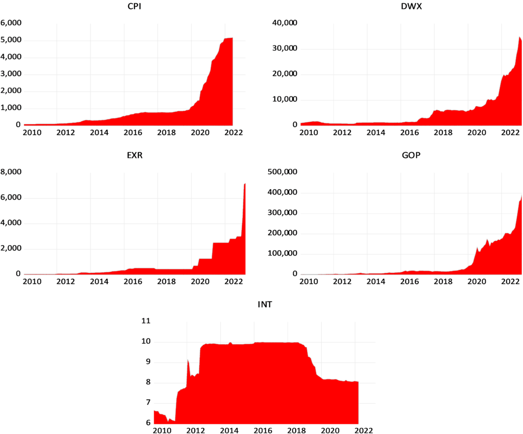
Figure 2. Evolution of high frequency study variables
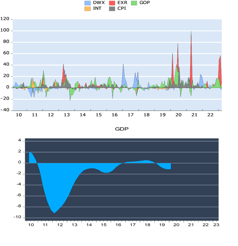
Figure (3) shows the magnitude growth of the macroeconomic and financial variables in Syria during the indicated period. We note that the data is characterized by the lack of a general trend and volatility around a constant. We found that the fluctuations change over time and follow the characteristic of stochastic volatility that decreases, increases and then decreases. We found that the most volatile variable is the exchange rate (EXR) and the period between 2019 and 2020 is the one when the variables fluctuated the most due to uncertainty and US economic sanctions. We also noted that the periods of high volatility are offset by negative growth in Syria’s GDP. Using the following Table (2), we show the most important descriptive statistics for the study variables.

*** denotes the significance of the statistical value at 1%. ** at 5%. * at 10%.
Table (2) shows that the probability value of the normal distribution test statistic is significant at 1%, and we conclude that the data on the growth rates of the Syrian economy is not distributed according to the normal distribution, and both the mean and the standard deviation were not useful for the prediction in this case since they have become a breakdown. We also note from Table (2) the positive value of the skewness coefficient for all variables, and therefore the growth rates of economic variables are affected by shocks in a way that leads to an increase in the same direction, except for the economic growth rate, in which the shocks are negative and the distribution is skewed to the left. We also found that the value of the kurtosis coefficient is high (greater than 3 for all variables), indicating a tapered leptokurtic-type peak. Additionally, we noted that the largest difference between the maximum and minimum value of the variable is the exchange rate, which indicates the high volatility due to the devaluation of the currency with the high state of uncertainty after the start of the war in Syria. Also, one of the key characteristics of growth rates is that they are stable (i.e. they do not contain a unit root). Since structural changes affect expectations, as we have seen in Figure (1), there is a shift in the path of the variable due to political and economic events. We hence used the breakpoint unit root test proposed by Perron et al [49-50], where we assume that the structural change follows the course of innovation events and we test the largest structural breakpoint for each variable and get the following results:
![]()
Where is break structural coefficients, is dummy variable indicated on structural change, : intercept, : lag degree for AR model. Figure (4) shows the structural break estimate for the study variables. Structural break refers to a change in the behavior of a variable over time, shifting relationships between variables. Figure (4) also demonstrates that all macroeconomic variables have suffered from a structural break, but in different forms and at different times, although they show the impact of the same event, namely the war in Syria and the resulting economic blockade by Arab and Western countries, as all structural breaks that have occurred after 2011. We found that in terms of the rate of economic growth, it has been quickly influenced by many components and patterns. For EXR, CPI, GOP, the point of structural change came after 2019, the imposition of the Caesar Act and the Corona Pandemic in early 2020, which resulted in significant increases in these variables. We noted that the structural break in the Damascus Stock Exchange Index has occurred in late 2016 as the security situation in Syria improved, resulting in restored investor confidence and realizing returns and gains for the market.
The step involves imposing the initial information on the structure of the model according to the properties of the data. Based on the results of the exploratory analysis, the prior Minnesota distributions were considered a baseline, and the main parameter is included in the hierarchical modeling:
Rho H = 0.2 is high frequency AR(1), Rho L = 0 is low frequency AR(1), Lambda = 5 is overall tightness, Upsilon HL = 0.5 is high-low frequency scale, Upsilon LH = 0.5 is low-high frequency scale, Kappa = 1 is exogenous tightness. C1 = 1 is residual covariance scale. The number of observations in the frequency conversion specifies the number of high frequency observations to use for each low frequency period. When dealing with monthly and quarterly data, we can specify that only two months from each quarter should be used. Last observations indicate that the last set of high-frequency observations from each low-frequency period should be used. Initial covariance gives the initial estimate of the residual covariance matrix used to formulate the prior covariance matrix from an identity matrix, specifying the number of Gibbs sampler draws, the percentage of draws to discard as burn-in, and the random number seed. The sample is divided into 90% training (in–of –sample) and 10% testing data (out-of–sample).
![]()
Table (3) provides us with the results of estimating the model to predict quarterly GDP in Syria. The results show the basic information to estimate the prior and posterior parameters, and the last section shows the statistics of the models such as the coefficient of determination and the F-statistic. We note that every two months were determined from a monthly variable to forecast each quarter of GDP in the BMFVAR model. Although there is no explanation due to the imposition of constraints, the model shows good prediction results with a standard error of less than 1 for each parameter and a high coefficient of determination of the GDP prediction equation explaining 93.6% of the variance in GDP.

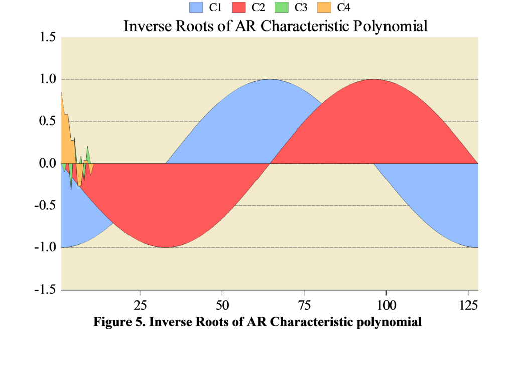
Figure (5) also shows us the reliability of the prediction results. It is clear that the roots of the estimation of the parameters follow the inverse AR polynomial process. The inverted AR roots have modules very close to one which is typical of many macro time series models.
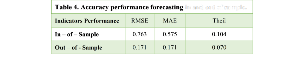
Table (4) shows the evolution of GDP Forecasting in Syria in and out the sample based on a number of indicators. When the value of these indicators is close to 0, the estimated values are close to the actual values, which is shown by Table 4, since the values of these indicators are all less than 1. The out-of-sample predicted values show a better performance of the model, and hence it can be adopted to track changes in quarterly GDP over time. Up-to-date with current versions.
Through the data visualization technique, Figure (6) shows us the closeness of the expected values of quarterly GDP in Syria in of sample, which leads to the exclusion of the presence of an undue problem in the estimate (overfitting – underfitting). The median is used in the prediction because it is immune to the values of structural breaks and the data are not distributed according to the normal distribution. The out-of-sample forecast results (Fig 7) also indicate negative rates of quarterly GDP growth in Syria with the negative impact of internal and external shocks on the Syrian economy with the accumulation of the impact of sanctions, the lack of long-term production plans and the ineffectiveness of internal monetary policy tools, as the latest forecasts for GDP growth this quarter are (-3.69%).
The uncertainty at each point in time is included in the Syrian GDP projections, thereby achieving two objectives: incorporating the range of GDP change at each point in time and knowing the amount of error in the forecasts. We found that uncertainty increases as the forecast period lengthens (Figures 8-10).
The model also provides us with important results through scenario analysis. Figure 11 shows that the quarterly GDP in Syria is affected by the shocks of high-frequency variables, since this Figure shows that the shocks have negative impacts. This recommends a better activation of the instruments of The Central Bank and those responsible for monetary policy in Syria. These results are considered important tools for them to know and evaluate the effectiveness of their tools.
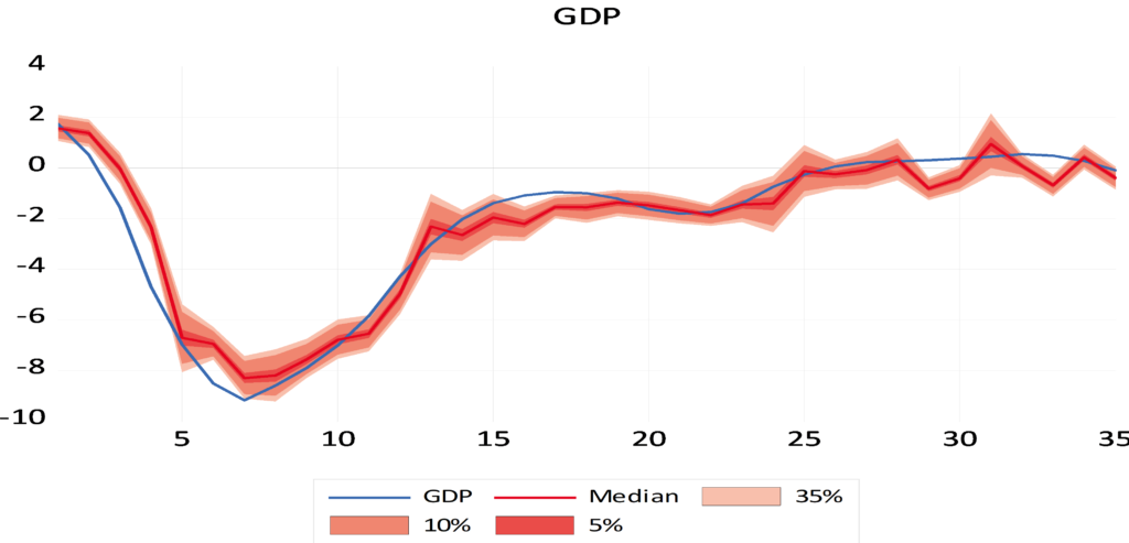
Figure 6. Forecasting quarterly GDP in Syria in of sample with 35%, 10%, 5% distribution quantities.
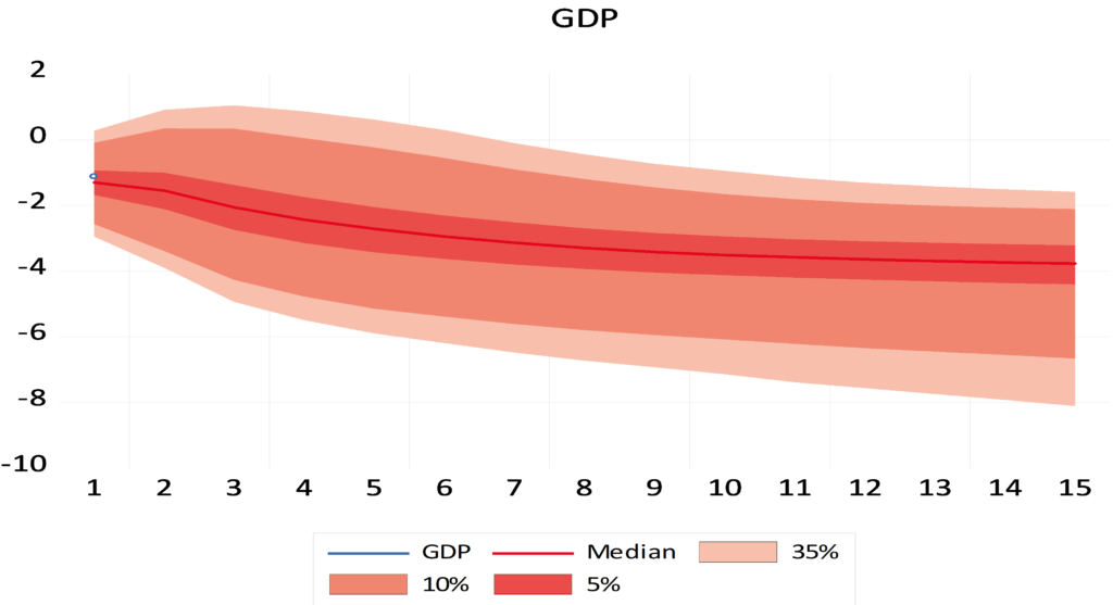
Figure 7. Forecasting quarterly GDP in Syria out of sample with 35%, 10%, 5% distribution quantities.

Figure 8. Uncertainty for forecasting quarterly GDP in Syria in-of –sample
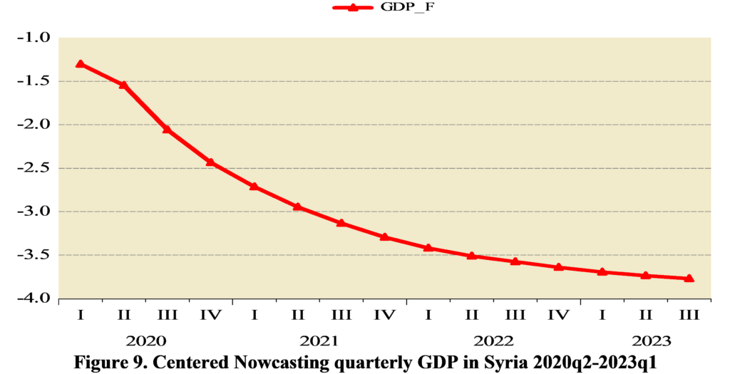

Figure 10. Uncertainty for forecasting quarterly GDP in Syria out-of –sample
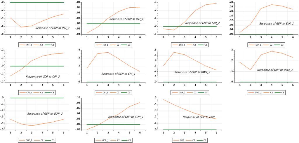
Figure 11. Shocks of high-frequency variables in the quarterly GDP of Syria
CONCLUSIONS AND RECOMMENDATIONS
This paper showed that BMFVAR could be successfully used to handle Parsimony Environment Data, i.e., a small set of macroeconomic time series with different frequencies, staggered release dates, and various other irregularities – for real-time nowcasting. BMFVAR are more tractable and have several other advantages compared to competing nowcasting methods, most notably Dynamic Factor Models. For example, they have general structures and do not assume that shocks affect all variables in the model at the same time. They require less modeling choices (e.g., related to the number of lags, the block-structure, etc.), and they do not require data to be made stationary. The research main finding was presenting three strategies for dealing with mixed-frequency in the context of VAR; First, a model – labelled “Chow-Lin’s Litterman Method” – in which the low-frequency variable (Gross Domestic Product) is converted from annual to quarterly with the aim of reducing the forecast gap and tracking the changes in the GDP in Syria in more real-time and reducing the gap of high-frequency data that we want to predict usage. Second, the research adopts a methodology known as “blocking”, which allows to treat higher frequency data as multiple lower-frequency variables. Third, the research uses the estimates of a standard low-frequency VAR to update a higher-frequency model. Our report refers to this latter approach as “Polynomial-Root BVAR”. Based on a sample of real-time data from the beginning of 2010 to the end of the first quarter of 2023, the research shows how these models will have nowcasted Syria GDP growth. Our results suggests that these models have a good nowcasting performance. Finally, the research shows that mixed-frequency BVARs are also powerful tools for policy analysis, and can be used to evaluate the dynamic impact of shocks and construct scenarios. This increases the attractiveness of using them as tools to track economic activity for both the Central Bank of Syria and the Central Bureau of Statistics.


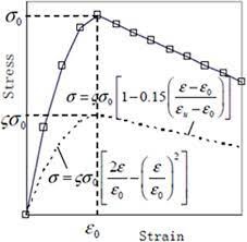


 Therefore, the proposed general mathematical formula could be expressed with the values of constant b in the ascending and descending parts of the curve.