Inverse Differential Control of a 6-Dof Parallel Manipulator Using Neural Networks


INTRODUCTION
Single image super-resolution (SISR) is a fundamental task in computer vision aimed at recovering high-resolution details from low-resolution input images [1]. It plays a crucial role in various applications, including surveillance, medical imaging, and satellite imagery, where obtaining high-quality images is essential [1]. Over the years, numerous methods have been developed to tackle the SISR problem, with the Super-Resolution Convolutional Neural Network (SRCNN) being one of the most prominent approaches [1]. SRCNN revolutionized the field of SISR by leveraging the power of deep neural networks to learn the mapping between low-resolution and high-resolution image patches [1]. By training on a large dataset of paired low-resolution and high-resolution images, SRCNN demonstrated impressive results in terms of reconstructing detailed and perceptually pleasing high-resolution images. However, SRCNN operates using real-valued neural networks, which may not fully capture the complex nature of image data [2]. In recent years, there has been growing interest in complex-valued neural networks as a potential enhancement to traditional real-valued networks. Complex-valued neural networks extend the capabilities of their real-valued counterparts by incorporating complex numbers as part of their computations [2]. This extension allows complex-valued networks to capture and process both magnitude and phase information present in complex data distributions. When applied to SISR, complex-valued neural networks offer several potential advantages. Firstly, they can better model the complex relationships and structures inherent in high-resolution images. By considering both real and imaginary components, complex-valued networks can effectively capture the intricate details and textures that contribute to the high-frequency information in an image. This property is particularly beneficial when handling images with fine textures, edges, and patterns [3]. Secondly, complex-valued neural networks have the potential to improve the preservation of image content during the super-resolution process. The ability to represent both magnitude and phase information enables complex-valued networks to better handle the phase shift problem that often arises in SISR. This issue occurs when the high-frequency components of an image are not accurately aligned during the upscaling process, leading to blurry or distorted results. Complex-valued networks can potentially mitigate this problem by explicitly modeling the phase information and preserving the integrity of the image content [4]. In short, the main contributions in this research paper are as follows:
The remainder of this paper is organized as follows. In Section 2, we provide an overview of related works in a single image super-resolution and complex-valued neural network. Section 3 presents the methodology, describing our case study SRCNN [1] and complex-valued neural network. In Section 4, we present the experimental setup and evaluate the performance of our method on a benchmark dataset. Finally, Section 5 concludes the paper.
RELATED WORK
In recent years, single-image super-resolution (SISR) techniques have garnered significant attention in the field of computer vision, aiming to enhance the resolution and quality of low-resolution images [1]. Traditional approaches relying on real-valued networks have faced inherent limitations in capturing complex image structures and relationships, prompting researchers to explore the potential benefits of complex-valued networks in SISR and other image-processing tasks [2]. Dong et al. [1] introduced the Super-Resolution Convolutional Neural Network (SRCNN), pioneering the application of deep learning for SISR and showcasing significant improvements in image reconstruction. Building upon SRCNN, subsequent approaches such as the Fast Super-Resolution Convolutional Neural Network (FSRCNN) [3] optimized network architectures for faster processing without compromising reconstruction quality. Additionally, very deep architectures like the Very Deep Super-Resolution (VDSR) network [4], the Enhanced Deep Super-Resolution Network (EDSR) [5], and the Residual Channel Attention Network (RCAN) [6] have achieved remarkable performance by leveraging residual learning and attention mechanisms. Advancements in generative adversarial networks (GANs) have led to the development of the Super-Resolution Generative Adversarial Network (SRGAN) [7], focusing on generating perceptually realistic high-resolution images. More recently, the exploration of complex-valued neural networks has shown promise, with studies by Li et al. [8], Xu et al. [9], and Zhang et al. [10], demonstrating superior performance in capturing complex image structures and relationships. Li et al. [11] investigated the use of complex-valued networks for image de-noising, demonstrating their effectiveness in modeling complex noise patterns. Xu et al. [12] proposed a complex-valued neural network architecture for SISR, preserving phase information during the super-resolution process for sharper and more accurate reconstructions. Moreover, Zhang et al. [13] introduced a complex-valued residual network for SISR, facilitating the learning of more expressive representations and achieving improved performance. The potential of complex-valued networks extends beyond SISR, as evidenced by studies in image painting [14] and multi-modal image fusion [15]. These findings underscore the promising role of complex-valued networks in overcoming the limitations of traditional real-valued networks and enhancing various image-processing tasks.
METHODOLOGY
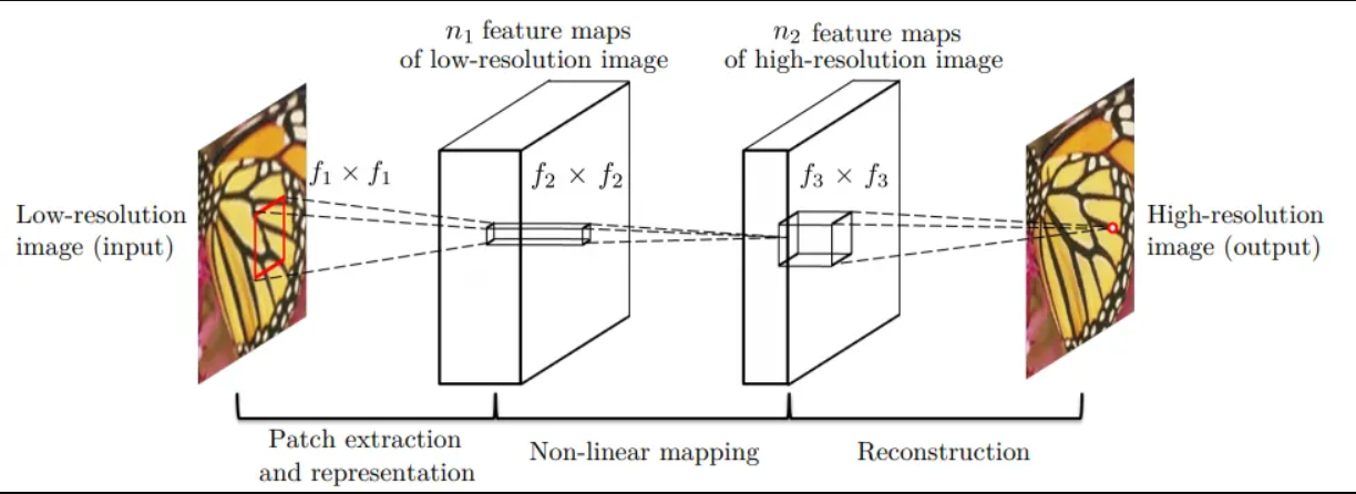
The Super-Resolution Convolutional Neural Network (SRCNN) is a deep learning-based technique designed for single image super-resolution (SISR). Originally introduced by Dong et al. in 2016 [1], SRCNN aims to learn the mapping between low-resolution (LR) and high-resolution (HR) image patches using a three-layer convolutional neural network (CNN). The network architecture of SRCNN comprises three primary stages (Fig 1): patch extraction and representation, non-linear mapping, and reconstruction. Each stage is detailed below:
Patch Extraction and Representation
In this initial stage, the low-resolution input image is divided into overlapping patches. These patches are the inputs to the SRCNN model and are represented as high-dimensional feature vectors. Let ILR denote the low-resolution input image, and f1 be the first convolutional layer with filter size f1×f1 and n1 filters. The output of this layer is:
F1=σ(W1∗ILR+b1)
where W1 and b1 are the weights and biases of the first layer, respectively, denotes convolution, and σ is the activation function.
Non-linear Mapping
The high-dimensional feature vectors from the first stage are input into a second convolutional layer that performs non-linear mapping. This layer uses a set of learnable filters to capture the complex relationships between the low-resolution and high-resolution patches. Let f2 denotes the filter size of the second convolutional layer with n2 filters. The output is given by:
F2=σ(W2∗F1+b2)
where W2 and b2are the weights and biases of the second layer.
Reconstruction
In the final stage, the feature maps from the non-linear mapping layer are processed by a third convolutional layer that aggregates the information to generate the high-resolution output. Let f3 denotes the filter size of the third convolutional layer with n3 filters. The high-resolution output image IHR is obtained as:
IHR=W3∗F2+b3
where W3 and b3 are the weights and biases of the third layer. The final high-resolution image is reconstructed by combining the outputs from all patches in the overlapping regions. By leveraging these three stages, SRCNN effectively transforms low-resolution images into high-resolution counterparts, enhancing image quality and details [1].
In this research, we propose a novel complex-valued neural network architecture for enhancing single image super-resolution (SISR). This approach builds upon the success of the Super-Resolution Convolutional Neural Network (SRCNN) model, but with a key distinction: we transformed the SRCNN architecture to incorporate complex-valued operations.
Traditional CNNs for SISR rely on real-valued numbers for computations. While these models have achieved significant results, recent research explores the potential of Complex-Valued Neural Networks (CVNNs) in this domain. CVNNs leverage complex numbers, which hold both magnitude and phase information, potentially offering advantages over real-valued approaches [16].
Natural images contain crucial phase information alongside magnitude. Standard CNNs primarily focus on magnitude, potentially losing details during super-resolution. CVNNs, by incorporating complex numbers, can explicitly handle both aspects, leading to potentially sharper and more accurate reconstructions [16].
Traditional SISR methods often suffer from phase shifts, introducing artifacts and distortions [17]. CVNNs, by explicitly dealing with phase information, can address this issue and generate more realistic super-resolved images.
The SRCNN model serves as a strong foundation for SISR tasks due to its effectiveness. However, to enable complex-valued computations within the network, we introduce several modifications and transformations to the original SRCNN architecture. These modifications are detailed below:
 where j is the imaginary unit [16].
Where and are the complex-valued weights and biases of the first layer, ∗ denotes convolution, and σ is the activation function applied to complex numbers [16, 17].
![]() where: d represents a complex-valued input.Re{d} and Im{d} denote the real and imaginary parts of d, respectively. j is the imaginary unit. ReLU is the standard Rectified Linear Unit activation function. CReLU’s simplicity and effectiveness make it a prevalent choice for complex-valued neural networks.
where: d represents a complex-valued input.Re{d} and Im{d} denote the real and imaginary parts of d, respectively. j is the imaginary unit. ReLU is the standard Rectified Linear Unit activation function. CReLU’s simplicity and effectiveness make it a prevalent choice for complex-valued neural networks.
Nearest Neighbor Upsampling (Mathematical Definition): For each new pixel location in the upsampled output, this method simply replicates the value of the nearest neighboring pixel in the original complex-valued input.
Bilinear Interpolation for Complex Data:
Bilinear interpolation for complex-valued data builds upon the concept of standard bilinear interpolation used for real-valued images. Here’s a breakdown of the general approach:
 where: L represents the CMSE loss value. Δx and Δy represent the differences between the real parts (x) and imaginary parts (y) of the predicted (zpredicted) and ground truth (zgt) complex numbers, respectively. By incorporating these modifications and transformations, our complex-valued neural network should be able to effectively capture the complex structures and relationships present in high-resolution images. This architecture enables the network to leverage the benefits of complex numbers and provide enhanced super-resolution capabilities compared to traditional real-valued networks.
Experimental Results
Dataset and Evaluation Metrics
To evaluate the performance of our complex-valued network (C-SRCNN) and compare it with the traditional SRCNN, we utilize standard benchmark datasets commonly used in single image super-resolution (SR) tasks. These datasets consist of diverse, high-resolution (HR) images paired with their corresponding low-resolution (LR) counterparts. The datasets are typically split into training, validation, and testing sets to ensure robust model evaluation.
We specifically chose a set of benchmark datasets encompassing various image types, including natural scenes, objects, and textures. This selection considers the potential increase in parameter size for our C-SRCNN due to its complex-valued nature compared to the real-valued SRCNN. This diversity allows us to assess the trade-off between achieving high reconstruction quality and model complexity. Additionally, it enables us to evaluate the generalization capability of C-SRCNN for handling different image content compared to the traditional SRCNN.
Here’s a detailed breakdown of the chosen benchmark datasets:
Set5: Contains 5 pairs of LR and HR images with a resolution of 256×256 pixels.
Set14: Contains 14 pairs of LR and HR images with a resolution of 512×512 pixels.
BSD100: Contains 100 HR images with a resolution of 512×512 pixels. Commonly used for SR tasks and other image processing applications.
Urban100: Contains 100 HR images with a resolution of 512×512 pixels captured from urban scenes.
To quantify the performance of our models, we employ standard metrics used in SR tasks: Peak Signal-to-Noise Ratio (PSNR) and Structural Similarity Index Measure (SSIM). Higher PSNR values indicate better image quality by measuring the ratio between the reconstructed image’s signal and noise. SSIM goes beyond just intensity differences and considers structural similarities between the reconstructed image and the ground truth, providing a more comprehensive evaluation.
Training and Evaluation
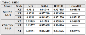
We used the T91 training set, which consists of 91 images, to train C-SRCNN. To ensure the generalizability of our C-SRCNN, we evaluated it on multiple standard benchmark datasets commonly used in single image super-resolution (SR). These datasets include Set5, Set14, BSD100, and Urban100. We compared the performance of our C-SRCNN against its real-valued counterpart, R-SRCNN. The training was conducted on a computer running Linux Ubuntu 18 with an Nvidia GTX 1060 GPU.steps =200000 and epochs = 219 patch = 128 . The quantitative results are presented in Table 1 and Table 2. Our proposed method achieved superior PSNR and SSIM scores on all four datasets compared to SRCNN-915. The PSNR results indicate an improvement of 0.435 for CSRCNN-915.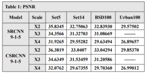
In addition, the SRCNN network was trained using different filter sizes in each layer. The number of parameters for each network was compared, and the results showed that the C-SRCNN network outperformed despite having fewer parameters. This highlights the effectiveness of the complex-valued network architecture in extracting image features, leading to superior performance. In conclusion, the results in Table 3 strongly support the efficacy of the C-SRCNN architecture for enhancing single-image super-resolution. This approach demonstrates the potential of complex-valued networks to achieve high-quality results with more efficient parameter usage.
Subjective visual assessment demonstrates the effectiveness of the C-SRCNN algorithm in enhancing the quality of single-image super-resolution (SISR) images. This algorithm excels in preserving detail sharpness, color accuracy, and noise reduction compared to the Real-SRCNN algorithm.
By utilizing these evaluation metrics, we can objectively assess the performance of our complex-valued network in enhancing single-image super-resolution. We compare the results obtained from our complex-valued network with those achieved by the traditional SRCNN. This comparison allows us to determine the effectiveness of the complex-valued network architecture in capturing complex image structures and improving the overall quality of super-resolved images.
RESULTS AND ANALYSIS
The transformation of SRCNN with complex-valued neural networks offers several benefits. Firstly, it allows for better preservation of fine details and textures during the super-resolution process. The complex-valued convolutions enable the network to capture subtle variations in color and texture, resulting in more visually appealing and realistic high-resolution images. Additionally, the complex-valued network can handle complex-valued input data, making it suitable for applications involving complex image representations. However, there are also challenges associated with complex-valued neural networks, including increased computational complexity and the interpretability of complex-valued networks may be more challenging compared to real-valued networks. In the future, researchers can focus on developing more efficient training algorithms and exploring novel architectures that leverage the power of CVNNs for SISR. Furthermore, the creation of comprehensive complex-valued data sets can facilitate the training and evaluation of CVNN-based SISR models.
CONCLUSIONS
Complex-valued CNNs present a promising avenue for advancing the field of image super-resolution. By incorporating complex-valued representations and making the necessary modifications, we can enhance the capabilities of CNNs for various image-processing tasks. The inclusion of magnitude and phase information, along with rotation and shift invariance, empowers the CV-CNNs to produce more accurate and visually appealing results. While challenges exist, further research and exploration of complex-valued CNNs hold great potential for improving image analysis and processing techniques.
INTRODUCTION
In recent years, deep learning models have exhibited remarkable performance in numerous Natural Language Processing (NLP) tasks, such as parsing [1], text classification [2], [3] and machine translation [4]. These models are typically characterized by their substantial parameter count, often reaching millions, necessitating extensive data for training to prevent overfitting and enhance generalization capabilities. However, collecting a sizable annotated dataset proves to be a laborious and costly endeavour. To mitigate the data-hungry nature of deep learning models, an approach known as automatic data augmentation has emerged. This technique involves generating synthetic data samples to augment the training dataset, effectively serving as regularization for the learning models. Data augmentation has been actively and successfully employed in computer vision [5], [6], [7] and speech recognition tasks [8], [9]. In these domains, methods frequently rely on human knowledge to apply label-invariant data transformations, such as image scaling, flipping, and rotation. However, natural language processing presents a different challenge, as there are no straightforward rules for label-invariant transformations in textual data. Even slight changes in a word within a sentence can drastically alter its meaning. Consequently, popular data augmentation techniques in NLP focus on transforming text through word replacements, either using synonyms from manually curated ontologies, such as WordNet [10] or leveraging word similarity measures [11], [12]. Nonetheless, this synonym-based approach can only be applied to a limited portion of the vocabulary since finding words with precisely or nearly identical meanings is rare. Furthermore, certain NLP data augmentation methods are specifically designed for particular domains, rendering them less adaptable to other domains [13]. As a result, developing more versatile and effective data augmentation techniques remains a significant research challenge in the field of NLP. In recent researches, a straightforward yet highly impactful data augmentation technique called Mixup [7] has been introduced, demonstrating remarkable effectiveness in improving the accuracy of image classification models. This method operates by linearly interpolating the pixels of randomly paired images along with their corresponding training targets, thereby generating synthetic examples for the training process. The application of Mixup as a training strategy has proven to be highly effective in regularizing image classification networks, leading to notable performance improvements. Mixup methodologies can be classified into input-level Mixup [14], [15], [16] and hidden-level Mixup [17] depending on where the mix operation occurs. In the context of natural language processing (NLP), applying Mixup poses greater challenges compared to computer vision due to the discrete nature of text data and the variability in sequence lengths. As a result, prior efforts in Mixup for textual data [18], [19] have put forth two strategies for its application in text classification: one involves performing interpolation on word embedding, while the other applies it to sentence embedding. This incentive drives us to explore Mixup text techniques for low-resource languages, specifically concentrating on Arabic sentiment classification. Our study involves a comparative analysis of basic LSTM classification models, both with and without the incorporation of Mixup techniques. Furthermore, we conduct experiments on diverse datasets, spanning sample sizes varying from hundreds to thousands per class. Additionally, we perform an ablation study to investigate the effects of different Mixup parameter values. To the best of our knowledge, this represents the pioneering research utilizing Mixup in the context of Arabic text classification.
MATERIALS AND METHODS
Mixup Concept
Define abbreviations and acronyms the first time they are used in the text, even after they have been defined in the abstract. Abbreviations such as IEEE, SI, MKS, CGS, sc, dc, and rms do not have to be defined. Do not use abbreviations in the title or heads unless they are unavoidable. The concept of Mixup involves creating a synthetic sample through linear interpolation of a pair of training samples and their corresponding model targets. To elaborate, let us consider a pair of samples denoted as (xi, yi) and (xj, yj), where x represents the input data, and y is the one-hot encoding representation of the respective class label for each sample. The process of generating the synthetic sample is as follows: where λ could be either fixed value in [0; 1] or it is sampled from Beta distribution with a hyper-parameter Beta (α; α). The synthetic data generated using this approach are subsequently introduced into the model during training, aiming to minimize the loss function, such as the cross-entropy function typically employed in supervised classification tasks. To achieve computational efficiency, the mixing process involves randomly selecting one sample and pairing it with another sample drawn from the same mini-batch.
Mixup for text classification
In contrast to images that comprise pixels, sentences are composed of sequences of words. Consequently, constructing a meaningful sentence representation involves aggregating information from this word sequence. In typical CNN or LSTM models, a sentence is initially represented as a sequence of word embedding and then processed through a sentence encoder. Commonly used sentence encoders include CNN and LSTM architectures. The resulting sentence embedding, generated by either CNN or LSTM, is subsequently passed through a softmax layer to generate the predictive distribution encompassing the possible target classes for making predictions. In [18], Guo introduced two variations of Mixup tailored for sentence classification. The first variant, referred to as wordMixup, employs sample interpolation within the word embedding space. The second variant, known as senMixup, performs interpolation on the final hidden layer of the network just before it is fed into the standard softmax layer to generate the predictive distribution across classes. Specifically, in the wordMixup technique, all sentences are first zero-padded to a uniform length. Subsequently, interpolation is performed for each dimension of every word within a sentence. Let us consider a given text, such as a sentence consisting of N words, which can be represented as a matrix B in an N × d form. Here, each row t of the matrix corresponds to an individual word, denoted as Bt, and is represented by a d-dimensional vector obtained either from a pre-trained word embedding table or randomly generated. To formalize the process, let (Bi, yi) and (Bj, yj) be a pair of samples, where Bi and Bj represent the embedding vectors of the input sentence pairs, and yi and yj correspond to their respective class labels, represented in a one-hot format. For a specific word at the t-th position in the sentence, the interpolation procedure is applied. The process can be formulated as:
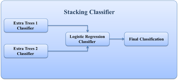
The obtained novel sample〖(B ̃〗^ij;y ̃^ij) is subsequently employed for training purposes. As for senMixup, the hidden embeddings for both sentences, having identical dimensions, are initially generated using an encoder like CNN or LSTM. Following this, the pair of sentence embeddings, f(Bi) and f(Bj), is linearly interpolated. In more detail, let f represent the sentence encoder; thus, the sentences Bi and Bj are first encoded into their corresponding sentence embedding, f(Bi) and f(Bj), respectively. In this scenario, the mixing process is applied to each kth dimension of the sentence embedding as follows. The sentMixup usually applies Mixup directly before the softmax while we experimented with an additional Mixup type that works on the hidden layers output similar to [17] applying Mixup before the final linear layer. Th proposed models’ structures are represented in Fig. 1.
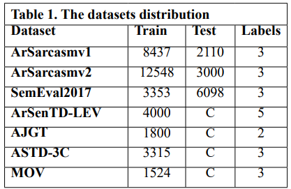
We performed experiments using 8 Arabic sentiment classification benchmark datasets: ArSarcasm v1 [36] & v2 [37], SemEval2017 [38], ArSenTD-LEV [39], AJGT [40], ASTD-3C [41], MOV [42]. The training sets differ in size (from 12548 to 1524), and in number of labels (2 to 5). The used datasets are summarized in Table 1.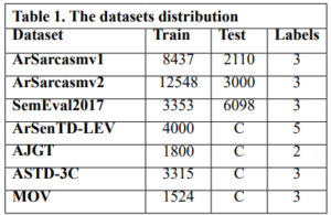 Preprocessing
The effectiveness of sentiment analysis models greatly depends on the quality of data preprocessing, which is equally critical as the model’s architectural design. Preprocessing involves cleaning and preparation of the text data for the classification process. Textual data, particularly when sourced from the internet, tends to be unstructured, necessitating additional processing steps for proper classification. The noise removal step during text data preprocessing involves eliminating several elements to enhance data quality. These elements encompass punctuation marks, numbers, non-Arabic text, URL links, hashtags, emojis, extra characters, diacritics, and elongated letters. Regular expressions serve as the primary technique for noise removal, effectively filtering out unwanted text.
Experimental environment and hardware
The experiments were developed using Python 3.9.7. The experiments, including their development, implementation, execution, and analysis, were conducted on an ASUS ROG G531GT Notebook. This machine runs Windows 11 and is equipped with a 9th generation Intel Core i7 processor, 32GB of RAM, a 512GB NVMe SSD, and an NVIDIA GeForce GTX 1650 4GB graphics card. The software libraries used in this study include PyTorch, Scikit-learn, Pandas, Gensim, and NumPy.
Model
We conducted an evaluation of wordMixup and senMixup using both CNN and LSTM architectures for sentence classification. In our setup, we employed filter sizes of 3, 4, and 5, each configured with 100 feature maps, and a dropout rate of 0.5 for the baseline CNN. For the LSTM model, we utilized 3 hidden layers, each comprising 100 hidden state dimensions, with the activation function set to tanh. Additionally, the mixing policy parameter is set to the default value of one. In cases where datasets lacked a standard test set, we adopted cross-validation with a k-fold value of 5 and reported the average performance metrics. Our training process utilized the Adam optimizer [36] with mini-batches of size 32 with 30 epochs and a learning rate of 1e-3. For word embedding, we employed 100-dimensional Aravec embedding.
DISCUSSION
Across the datasets, it is evident that applying Mixup techniques generally leads to slight improvements in accuracy compared to the baseline None model. However, the effectiveness of Mixup varies depending on the dataset. For instance, on the AJGT dataset, all Mixup variants consistently outperform the None model, with Mix-encoder and Mix-output achieving the highest accuracy of 85.2%. On the other hand, for the SemEval2017 and ArSenTD-LEV datasets, Mixup provides only marginal gains, suggesting that the impact of Mixup might be more prominent in certain scenarios. Additionally, while Mixup seems to be beneficial in some cases, it does not necessarily lead to performance improvements across all datasets. For instance, on the MOV dataset, the Mixup variants show comparable or slightly worse results compared to the None model. Furthermore, it is worth noting that the Mix-encoder and Mix-output models tend to perform better than the Mix-embed model in most cases. This could be attributed to the advantage of applying Mixup at the higher levels of the model architecture, which allows the model to capture more abstract and meaningful patterns. Mixup augments data by interpolating sequences, which can create new variations that capture a broader range of sequential patterns. LSTMs, with their capability to understand and generalize sequences over long contexts, can leverage these variations more effectively than CNNs, which focus more on local patterns and may not fully utilize the sequential nature of the augmented data. Overall, these results demonstrate that Mixup techniques can be advantageous to sentiment analysis tasks, but their effectiveness is influenced by the dataset characteristics and the specific Mixup strategy used.
CONCLUSIONS AND RECOMMENDATIONS
Taking inspiration from the promising results of Mixup, a data augmentation technique based on sample interpolation used in image recognition and text classification, we conducted an investigation into three variations of Mixup for Arabic sentiment classification task, which is the first study on Mixup in Arabic to our knowledge. Our experiments demonstrate that the application of Mixup leads to improvements in accuracy and Macro F1 scores for both CNN and LSTM text classification models. Notably, our findings highlight the effectiveness of interpolation strategies as a domain-independent regularizer, effectively mitigating the risk of overfitting in sentence classification. These results underscore the potential of Mixup as a valuable tool in the field of NLP for enhancing model generalization and performance across various sentence classification tasks. In our future research endeavors, we have outlined our intentions to explore and examine further proposed variations of Mixup. Among these variants are AutoMix [44], a method that adaptively learns a sample mixing policy by leveraging discriminative features, SaliencyMix [32], which synthesizes sentences while maintaining the contextual structure of the original texts through span-based mixing and EMTCNN [45], an Enhanced Mixup that leverage transfer learning to address challenges in Twitter sentiment analysis. We are also interested in questions related to the visual appearance of mixed sentences and the underlying mechanisms responsible for the efficacy of interpolation in sentence classification. These inquiries will provide valuable insights into the potential applications and benefits of various Mixup techniques, contributing to the advancement of NLP tasks, particularly those focused on sentence classification.

INTRODUCTION
Banning nationally generated certificates that do not have approved global security certificates is a major and fundamental problem in countries that fall under the technical and information ban, such as Iran, Syria, etc., this matter is considered as a paralysis of development wheel in most fields because the aspects of life today have become dependent on electronic transactions, such as: banking sector, electronic transfers and linking them to electronic payment cards, electronic transaction systems, applications that transfer data with a certain degree of confidentiality, custom query systems, web control systems, web ordering systems, all transactions related to electronic government … and other many uses. The root certificate for the root certification authority is issued within a highly protected information environment or system and is used to issue digital certificates to individuals or companies. These certificates and their keys are stored and saved within its private system or environment, and thus the CA is the trusted third party to verify the authenticity of the certificates or signatures that are signed with them. By using the root certificate, verification can be performed, and this is known as the concept of a national certification authority. The National certification authority is considered the cornerstone of everything related to possible applications and projects, including digital transformation, provision of electronic government services (government and civil transactions), electronic payment methods, exchange, approval, authentication and protection of documents, electronic identity, electronic passport, online elections and their integrity, etc. All of these applications or projects depend on the presence of digital certificates signed by the certification authority that issues the digital certificates. Note that these applications or projects require high capabilities to issue digital certificates to all members of the public, as the policy has been adopted in most countries. The National Digital Certification Authority project has not been invested in the optimal way planned for several reasons, the most important of which are: The technological ban on our country, Syria, as the Syrian digital certificate issuing authority is not recognized internationally, and therefore it has not obtained a signature from the global digital certification authorities that are recognized by well-known international browsers. And the inability of well-known international browsers to run applications working on the webs that use nationally generated certificates due to their failure to recognize these certificates because well-known international authentication companies do not certify these national certificates, due to the imposition of technological sanctions on our country and also on many countries that are under the ban. From the above, the need to have a web browser that can verify the authenticity of these certificates in a safe and reliable manner (safety secure way) without the need for authentication from global authorities arose (Certification Authorities). In order to build a web browser that can verify the authenticity of national digital certificates, it requires cooperation between governments and technology companies. Indeed, an agreement had previously been reached between the Network Services Regulatory Authority and a company to build a national web browser, but the project was not completed. In general, it can be said that building a web browser that can verify the authenticity of national digital certificates is necessary to solve the ban problem imposing on certificates, and gives individuals and organizations confidence in using national digital certificates for many purposes. As technology develops and more security technologies become available, this type of browser can be improved and developed to ensure that data security is maintained and authentication is confirmed in a safe and reliable manner, which is an important step in developing and improving the digital infrastructure of countries and individuals, and can help achieve the global goal of maintaining digital security and achieving digital integration between countries, institutions and individuals.
MATERIALS AND METHODS
First, we conducted analytical studies based on field visits to the Ministry of Communications and Technology, the National Authority for Information Technology Services, the government sector, and the private sector to understand the existing problem and discuss it with stakeholders. We also depended on reference studies through books and the Internet about the use of the /SSL, TLS/ protocol in browsers and how this is done through the national digital certificate issuance authority. We followed an inductive research methodology to collect and analyze information, as well as using programming and practical experience to design and develop the national browser. We have depended on a set of programming tools for programming development, which are: Programming by java in Intellij IDE – Programming by java netbeans IDE In addition to a virtual operating system environment on the server VMware Esxi7 (platform virtualization software) Which contains: linuxubuntu server 22.04 operating system. The system for generating digital certificates (Openxpki) wasinstalled, prepared and authenticated, the Windows Server 2022 operating system, where the Wireshark network monitoring tool was installed on it. In order to test the browser’s operation, we used a set of tools: Openxpki which is an open-source tool used globally to generate certificates of all kinds, as it is installed on the Apache web server within the Linux server operating system. A website on which a generated and nationally signed certificate is installed, and Wireshark, a tool used to monitor all network details, including data. The purpose of using it was to indicate whether the connection was successful and the data was encrypted through the https protocol when using national certificates, in addition to national certificates generated and signed by the National Authority for Information Technology Services.
RESULTS
Through this research, we found a solution to the ban problem by creating an open-source software application (web browser), as this browser allows the use of digital certificates approved by the National Authority for Information Technology Services. Other tasks can be added to the browser related to privacy and protection (for example, software code can be added to the browser so that it is linked with a specific web application in order to perform a specific task that may be related to privacy, Property protection, or preventing the use of the application except through this version of the browser…).
DISCUSSION
Description of the X.509 standard:
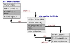
The X.509 standard consists of a set of rules and instructions that determine the method of issuing digital certificates and authenticating digital identity. The X.509 standard is considered the approved reference within the National Digital Certification Authority in Syria. The standard includes detailed information about the entity issuing the certificate and the entity in which the certificate was used, including digital identity information and the keys used in digital signature and encryption. The certifications that depend on X.509 standard are used to authenticate the identity of users, devices, and organizations, by including the digital identity information of the entity issuing the certificate. In general, the X.509 standard forms an important basis for maintaining digital security and authenticating digital identity, as it is used in many different security applications and can be used in many industries and sectors including e-government, e-commerce, banking services, and others. This standard was chosen in our research based on the reference study [1] which confirmed that this standard is used in the majority of global browsers. It analyzed the structure of this standard and how to benefit from it to ensure the identity of servers and the confidentiality of data exchange. The structure of the X.509 standard is illustrated in Figure (3).
Solve the problem by building a national web browser:
A browser was built in the Java programming language that can browse websites using the HTTPS protocol [5]. The browser interfaces were created that resemble the interfaces of well-known international browsers, in addition to building a private trusted certificate store (TrustStore [4]), where trusted certificates are supplied to it through two methods:
Then we tested the readiness of the trusted certificate store. After that, it was adopted as the default store of the national browser instead of the trust store of the operating system. The certificates included in the Trust Store, including the approved nationally generated certificates, can be viewed in Figure (2).
How the browser verifies the validity and reliability of the certificate:
When you browse a secure site (sites that start with the prefix “https://”) instead of “http://”), the browser uses a security protocol called SSL/TLS (Secure Sockets Layer/Transport Layer Security) to secure the connection between the browser and the server [10]. An SSL/TLS certificate is used to authenticate the server’s identity and encrypt the data that is exchanged between the browser and the server. To verify the validity of the certificate, the browser checks the existence of the certificate and whether it was sent by the server. The browser then verifies that the certificate has been signed by a trusted certificate authority (CA) located within the TrustStore [4] that the browser uses, and that the server’s name included in the certificate matches the server’s name in the URL being browsed. Then the browser determines the server’s address of the Online Certificate Status Protocol (OCSP) and the Certificate Revocation List (CRL) server’s address in the digital certificate file that is signed by the certificate issuing institution [10]. The validity of the certificate is checked for revocation or expiration in one of the following two ways:
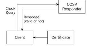
The OCSP server responds to the request after verifying the validity of the certificate. If the certificate is valid, a positive response is returned confirming its validity, and if it is invalid, a negative response is returned indicating its invalidity. As shown in Figure (4):

By using Certificate Revocation List (CRL), this method includes the following steps:
![Structure of the X.509 standard [researchgate.net]](https://journal.hcsr.gov.sy/wp-content/uploads/2024/03/Structure-300x164.jpg)
OCSP protocol differs from CRL protocol in the following way:
Comparison between the concepts of Keystore and Truststore [4]:
 How to test whether the browser is working properly:
In cooperation with the Digital Certification Center of the National Authority for Information Technology Services within the Ministry of Communications and Technology, an experimental website was developed (https://tools.ecc.sy) on the Internet, embedded with a generated and nationally certified certificate, and its operation was tested on three well-known browsers (MicrosoftEdge، Google Chrome، Mozilla firefox), These browsers were unable to run it due to the existence of the Syrian certificate, which is not trusted by them due to sanctions. The website was tested using the browser that was built and it worked. After running the experimental site on the national browser, the connection was tested if it is secure (encrypted) using the programming code which is custom of testing Https connection. In addition to testing the reliability of the certificate through the browser’s trust store, note that the success of the secure connection is shown by the appearance of a closed lock symbol and writing (Https status: ok) next to the address field within the browser. You can view the certificate for the experimental site described in paragraph 1 above and view the certifying parties (certificate authorities) for this certificate (chain of trust), in Figure (6).
The previous figure shows that the issuer name shown by the number (3) has certified the issuer name shown by the number (2), which in turn has certified the certificate for the experimental site on the Internet shown in number (1). The issuer name (certification authority) shown in the number (1) represents the national Syrian root certificate and is embedded in the browser’s trust store. Accordingly, the experimental site’s certificate was trusted and approved within the HTTPS protocol. When running a site that does not have a certificate or uses the /http/ protocol, the browser will show that. The success of the TLS protocol was monitored through the Wireshark application, which eavesdrops on the entire network. Also monitor data movement (exchanged in encrypted form) across the network through the Wireshark application.
![Verify the certificate through CRL [10].](https://journal.hcsr.gov.sy/wp-content/uploads/2024/03/verify2-300x208.jpg)

CONCLUSION
By the end of the research, the first Syrian national web browser was completed that includes a trusted certificate store that ensures the operation of the https protocol, and offers a set of solutions to the existing problems due to the international technological ban on our country, Syria, and other countries, which prevents us at Syria from using the Internet or the Intranet in the field of reliable electronic dealing in all sectors on government websites which have the SY extension. This Syrian national web browser allows the use of digital certificates approved, generated and signed by the National Authority for Information Technology Services, which are not trusted internationally due to sanctions. Our web browser is a secure, open-source and it can be portable application that does not require installation [2]. Finally, this browser is useful to All entities in the public and private sectors that need to use digital authentication or need protection and reliability in the operation of their applications. In the first place, it will serve the Ministry of Communications and Technology, the National Authority for Information Technology Services in Syria, which presented the National Digital Authentication Project that faltered due to the international browsers not supporting Syrian digital certificates.
FUTURE WORKS
After achieving the desired objectives of the research, which we have mentioned in the context of this article, we can identify a set of recommendations such as: adding tasks related to privacy and protection to the browser, for example adding a digital signature and adding programming code that links the browser to an application for preventing the use of that application except through this version of the browser. The browser can be used as a secure means of communication by adding programming codes that enable communication and the exchange of files and messages. Finally many features can be added and customized when needed for example, adding monitoring features for monitor all types of sites and adding Advanced security and privacy features.

INTRODUCTION
Pollution is a major problem that modern societies suffer from. The presence of pollutants in water resources, especially fresh water, makes it a serious and defining problem for growth and life [1].Pollution issues are constantly exacerbated in Coastal areas because of the increasing of population density and human activities that pollute the environment and natural resources, including water sources and groundwater which represents the reserve stock of water used in various fields [2] Environmental pollution affects all elements of the living environment such as plants, animals and humans, as well as the composition of non-living nature elements such as air, water and land. This problem has exacerbated in recent decades and become a grave danger threatening all living organisms because of industrial development, technological progress, and the development of the human standard of living accompanying with the increasing in consumption and the growing dumping of waste in the environment [3, 4] Solid waste is considered one of the major environmental problems in urban areas, due to its direct impact on the quality of human life, the appearance of civilization, and the consequent serious negative impact on sustainable development [5]. Solid waste resulting from various human activities (production and consumption) has become a major threat to the environment and people because of the increasing quantities generated daily which exceed the ability of the environment to decompose and convert them into useful or harmless materials [4]. The increasing production of raw materials and their consumption contributed to the depletion of natural resources and caused continuous damage to the environment [3]. Every year, the production of raw materials destroys millions of hectares of land and trees and produces billions of tons of solid waste. It pollutes water and air [6], in addition to the pollution resulting from the production and use of energy needed to extract and manufacture materials [7]. Surface water bodies have been used for a long time, and are still used today, as places for discharging various human waste, which exacerbated the problem of fresh water pollution in rivers, lakes and water reservoirs due to a change in its physical, chemical or biological properties. In addition to the pollution caused by these wastes to groundwater when the leachate reaches it [8]. The presence of indiscriminate dumping near water resources (ground or surface) contributes to their pollution and the pollution of the environment in all its aspects, especially groundwater, which represents the reserve stock of water used in various fields affecting growth and life, [9 ,10]. In wet weather, the movement of chemical and biological pollutants of solid waste materials is active, their concentration increases at the bottom of the landfill [11]. Most of leachate coming out of the landfills increases during periods of precipitation. solid waste forms severe pollution sources due to the abundance and diversity of chemical elements emerging from them[12]. Problems with health and environment increase with the appearance of some heavy metals in the groundwater, as specialized references confirm that their presence (no matter how small) is linked to solid waste, as it is one of the most dangerous and toxic chemical pollutants for living organisms [13, 10, 14], and is characterized by its long-term persistence in the aqueous medium, which ranges from several months to several years [14, 15]. The development which Syria witnessed in recent decades has been accompanied by the emergence and exacerbation of environmental pollution problems, as the surface and groundwater in the country suffer from the accelerating rate of bacterial and chemical contamination with industrial, domestic, and fertilizer waste [5]. It has been shown that the pollution, and the amount of waste in general, has increased with the increasing in the population in the countryside and cities, because of the weakness of the treatment plants. [16]. One study also showed an increasing in bacterial population in the water of wells used to irrigate some vegetables near the waste dumping site in the Al-Bassa area in Lattakia during winter [17]. In the same context, the study of the environmental impact of the Al-Bassa landfill [18] concluded that some indicators of contamination of groundwater wells in the Al-Bassa area increased, and it was noted that the rates of BOD and NO3 increased above the permissible levels for drinking water. Another study showed bacterial and physiochemical contamination of the waters of the Al-Kabir Al-Shamali River in the Al-Jindiriya area [19]. The importance of this research lies in evaluating the quality of water in the wells located in the vicinity of Wadi Al-Hada Center, in addition to the clear environmental effects of waste leaching on some groundwater wells located in the vicinity of it, especially after the appearance of turbidity in two wells located in Beit Ismael and Minya Yahmour villages. The research aims to monitoring and evaluating the quality of groundwater within ten wells located in five villages adjacent to the center of Wadi Al-Hada by determining some physical and chemical characteristics of groundwater in two wells from each village for a period of four months (until the results of the analysis became identical to the Syrian standard specifications) and determining measures to reduce the impact of major water pollutants.
MATERIALS AND METHODS
Study site and sampling sites:
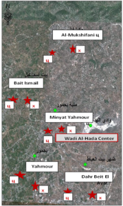
This research was conducted in the area surrounding the Wadi Al-Hada Center for Solid Waste Treatment, located in the village of Al-Fatasiyah, 13 km southeast of Tartous, and at an altitude of about 180 meters above sea level. The area of the center’s land is 100 dunums. several sites next to the center are used for dumping waste resulting from the center. The center is surrounded by a group of small villages and residential communities working in agriculture (these are the villages of Yahmour, Al Zarqat, Minyat Yammour, Karm Bayram, Beit Ismail, and others…) The irrigation of crops in these villages depends on groundwater. The idea of this research came from the appearance of detectable pollution in two wells located in Minyet Yahmour and Beit Ismail, due to exposure to waste leaching. The research was divided into two stages In the first stage, a survey was conducted by distributing questionnaires to local population. This questionnaire covered 50 families, and included questions to explore their opinions about the center, their health conditions, diseases suffered by family members, and the repercussions of water pollution on them due to the old dump and treatment center in Wadi al-Hada, and the availability of a sewage network in the area. In the second stage, the impact of Wadi Al-Hada center on some wells in five villages adjacent to it was studied as shown in Figure 1. Groundwater samples were taken from 10 artesian wells (Table 1) distributed in the region, so that they represent the various conditions of the site in terms of human activity and land use, and analyzes were conducted.
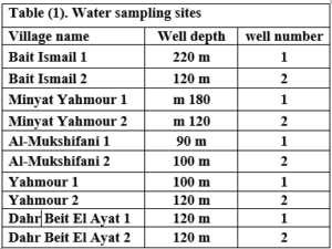 Several field visits were made to the study site, and water samples were taken from these wells six times, at an interval of ten to twenty days. The sampling was stopped when the results became in conformity with the Syrian standard specifications starting from 7/27/2021 until 10/12/2021. Sample collection and analysis: Samples were collected in 1-liter polyethylene containers to determine the COD index and measure some electrolytes. The containers were washed well with distilled water and study site water three times before being filled; other samples were collected in 500 ml glass containers to determine the number of faecal bacillus FC. The containers were sterilized in an oven at a temperature of 250ºC for two hours Water analyses were conducted in the laboratories of the Directorate of Water Resources in Tartous Governorate, as follow:
Working methods:
Physical, chemical and bacteriological analysis were carried out in the laboratories of the Directorate of Water Resources in Tartous, according to the following: Some physical indicators (pH, turbidity, and electrical conductivity) were measured at the study site using newly calibrated field devices as follows:
FC – (fecal coliform count): FC was determined using the filtration method on 0.45-micron bacterial membranes and incubated with MFC agar culture medium at 37.5°C for 24 hours using the following equipment: Bacterial isolation chamber from Lab Tech, buchner funnel for filtering bacterial samples, a bacterial incubator from Memmert, a sterilization oven from Memmert, and an autoclave from SELECTA, model AUTESTER ST
RESULTS
At the beginning of the research, the wells in Minyat Yahmour and Beit Ismael were polluted, due to the exposure of the aquifer to pollution by the waste leaching collected next to the center, but when the leachate was collected, the results returned to the permissible limits according to the Syrian standard specifications shown in “Table2”.
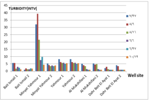
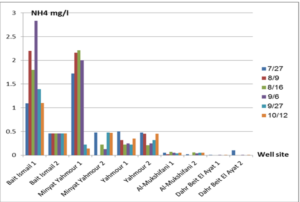
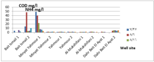
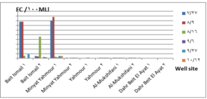
The pH values were moderate values tending to alkalinity, and were within the permissible limits according to the Syrian standard specifications and so was the electrical conductivity (Cond) which did not exceed 813 μM/cm in the wells. Whereas turbidity values were high in most of the wells in the first samples during July and August, especially in (well 2) Minyat Yahmour, where it reached (39ntu, 32ntu), and in (well 1) Yahmour (8ntu.2ntu) “Fig 2”. We also noted that the percentage of ammonia was above the permissible limits according to the Syrian standard specifications. “Fig 3”. COD values in all measurement locations exceeded the permissible limits according to the Syrian standard specifications (which is 2 mg/L) in the first samples, ( in July and August), “Fig 4”, and also the results of the bacteriological analysis showed high general count and a high number of coliform bacilli in the two wells located in Beit Ismail and well 2 located in Minyet Yahmour, “Fig 5” Finally, positive and negative electrolytes, It was noted that the values of the ions NO2-، NO3- ، PO43-، Cl-، SO42-did not exceed the permissible limits according to the Syrian standard specifications in the ten wells. Population survey results: The results of the questionnaire showed the occurrence of disease cases as a result of the use of contaminated well water.
DISCUSSION
We will graphically review only the indicators that do not conform to the Syrian standard specifications and analyze their changes spatially and temporally. The pH values were within the permissible limits according to the Syrian standard specifications. There was no significant change in them according to the change in the sampling date or the location of the well. As for turbidity, we noticed high turbidity values in most of the wells in the first samples, and we can attribute this to the leaching of pollutants from the landfill into the effluent that heads from Wadi al-Hada center towards Minyat Yahmour and Beit Ismail. Then, the values of turbidity decreased until it became within the permissible limits according to the Syrian standard specifications in November. This is because the problem was solved in the area and the leachate was collected in the rainwater collection basin and This is consistent with studies confirming the impact of landfill leachate on groundwater [20, 21] The measurements also indicated that the electrical conductivity values of well water and surface water were within the permissible limits according to the Syrian standard specifications (1500 µm/cm), but the ammonium ions in the water influenced by human activity as the nitrogen was presented in polluted water (urine and uric acid). The production of ammonium ion during the ammonification process indicates the recent existence of contamination with organic matter and the progress of the self-purification process that carried out by microorganisms in aquatic media. [22].COD values: It is noted from “Fig 4” that the COD index has increased, as the highest value was recorded in well 2 located in Minyet Yahmour and the two wells located in Beit Ismail, but these values began to decline until they became within the permissible limits in the month of November, and this indicated that the aquifer was contaminated with highly concentrated organic matter that may be due to the leachate from Wadi Al-Hada. The discrepancy in the results between the wells can be explained by the difference in the slope and permeability of the soil and rocks at this location compared to the locations of other wells [4] “Fig 5” shows the bacteriological analysis that it exceeded the permissible limit (which is zero) in all wells except for the (two wells) in Dahr Beit Al-Ayat and (well 1) in Minyet Yahmour,the value (zero) was recorded which was good . The largest value was in the two wells (well l) in Beit Ismail and ( well 2) in Minyet Yahmour, during the first three months (July, August and September). This may be due to the fact that there is sewage near them. As for the rest of the wells, the number of coliform bacilli was greater than zero, but it was relatively less than these wells and this is consistent with studies confirming the impact of waste leaching on the groundwater [23, 24] Positive and negative electrolytes: It was noted that the values of the ions NO2-, NO3-, PO43-, Cl-, SO42- did not exceed the permissible limits according to the Syrian standard specifications in the ten wells during the four months. This can be explained by the fact that they were not subjected to excessive fertilization, and this was indicated by many studies [25,26,27]; However, the results showed an increase in the concentration of ammonia ions in the two wells located in Beit Ismail and Minyat Yahmur. It was also found that there is no clear relationship between the depth of the well and the values of the pollution indicators in it. This can be attributed to the fact that the studied wells were not fed by the same aquifer [28]. It is important here to point out a study on Modeling the movement and transport of pollutants in the groundwater using GMS program (a quantitative model using MODFLOW, and a qualitative model using MT3D), which was conducted at (Al-Bassa Dump) [29], and the results of the quantitative modeling of the water resources system in the Al-Bassa Dump area resulted in obtaining a map of Head Contours and flow Budgets, and the ability to display cross-sections at any point of the studied area. We also were able, through qualitative modeling, to simulate the transport of pollutants, and the leakage of leachate from Al-Bassa Dump, and predict its expected changes during different periods. Therefore, it is necessary to emphasize the importance of using modeling programs to predict the movement of pollutants in the Wadi Al-Hada center area. Population survey results: The results of the questionnaire showed the occurrence of disease cases as a result of the use of contaminated well water, the most important of which were acute intestinal diarrhea and gastrointestinal infections. 30% of the surveyed people indicated that they were exposed to diseases because of the landfill or as a result of their use of groundwater wells, and most of them stopped using this water for drinking and only used it to irrigate crops. The results also showed that 80% of the population are farmers and have lived in the area for more than 50 years, and 25% of them depend on technical drilling.
CONCLUSIONS AND RECOMMENDATIONS
We can conclude from this study the following main points:
RECOMMENDATIONS
To avoid the health and environmental harms of the waste and sewage water, we recommend the following:
Use a modeling program to predict pollutants by constructing a mathematical model using GMS program (a quantitative model using MODFLOW, and a qualitative model using MT3D).
INTRODUCTION
Substitutes to cement are a sustainable way to decrease the overuse of cementitious materials, and it is gradually becoming important to include them in the building sector [1]. Energy consumption is the major environmental concern associated with cement manufacture, including the direct use of fuel to extract and transport the raw materials as well as the high energy required for calcination, which is provided by burning of coal, coke, natural gas, diesel and fuel. Cement manufacture consumes about 1758 kWh per ton of cement. Mortar is one of the decorative building elements in addition to its role as a binder for the block and is widely used in the construction field. The mortar mixture consists of Portland cement, fine aggregate, and water. Many adjustments have been made to the mortar concerning its components [2]. The various construction processes are one of the main sources of high carbon emissions, as the cement industry is a significant component in increasing carbon emissions. Using other cementitious materials to produce cement-based materials is an important technique to decrease carbon emissions, where the cement industry generates nearly 8% of global CO2 [1]. Fly ash and Silica fume (pozzolanic materials) are widely used as cement alternatives to produce cement-based materials [1]. The consumption of local raw resources is one of the obstacles to cement manufacture [3] [4]. In addition, issues related to climate change have attracted significant attention. However, more recently, issues related to local health aspects have been mentioned. Therefore, designers of building material mixtures seek to introduce sustainable technologies to reduce environmental impact [5] [6]. Current technological advances aim to improve the construction process in terms of speed, performance and financial productivity. The use of gypsum mixes that do not require high levels of heat during the production process is common [7]. Gypsum is a construction material known for its good performance against variations in humidity and its rapid ability to change shape and harden. However, gypsum materials have some disadvantages for use in construction, such as: not being hard or brittle, poor waterproofing and decomposing quickly. For this reason, many researchers have conducted numerous tests to determine and improve the performance of these materials. Archaeologists dated the earliest uses of gypsum about 7000 BC [8]. Many researchers aimed to replace raw building materials with wastes and biomass (low energy consumption binders) to increase the environmental efficiency of construction. Gypsum is considered one of these low-cost materials, that seems to be a suitable option for new constructions, in addition to being widely used in many restoration and rehabilitation operations for old buildings. The advantage in which gypsum is distinguished from cement and lime is its production at about 120-180 °C, with a much lower burning temperature and energy, while cement needs about 1500°C and lime needs about 900°C. Thus, the associated low energy makes gypsum a sustainable solution [9]. Concerning energy saving in buildings in European countries, around 75% of buildings need incomplete or complete repair because they are not energy efficient. Enhancing the performance of wall cladding (interior and exterior) is an important energy-saving technology as part of the rehabilitation and maintenance of damaged and older buildings [10]. As for Syria, this percentage increases very significantly as a result of the war that the country was exposed to, according to the observations of the authors themselves, to more than 90%. By the way, statistical reports issued by the International Energy Agency indicate that worldwide energy depletion in the building sector will reach 30% in 2060 if the existing ratio of increasing growth remains as it is now [11]. Accomplishing high energy efficiency in structures is the most demanding concern of governments internationally, which would cause a decrease in energy depletion and environmental problems related to CO2 emissions [11]. Various research projects and investigations began years ago to find suitable alternatives to reduce the concentration of carbon dioxide in the atmosphere, in addition to reducing the cost of building materials [12][13][14]. Unpredicted environmental hazards of carbon emissions resulting from cement manufacturing required for all structures in addition to depletion of raw resources are the most persistent tasks of future engineering. However, achieving sustainability by introducing natural materials that are affordable for various construction process is one of the preferable solutions. Due to the lack of searches done on JB, and its wide spread in the Deir ezzor region, it was necessary to draw attention to that product and define its specification. The key objective of this investigation is to determine the engineering properties of JB-based mortar. JB is used as a partial replacement of cement with varying ratios of 0%, 10%, 25%, 50% and 75% of the total cement weight. Then, comparative results between the cement mortars and JB-based mortar will be presented.
MATERIALS AND METHODS
JB: The southern region of Deir ezzor is generally famous as the extraction deposits of the raw material for the production of JB. A large number of limestone mountains, the most important of which are the southern mountains near the Qabr al-Wali area, the Hawooz area, the Tharda Mountains, and the ancient al-Jura area. A single limestone mountain mass is called a Maqtaa, it is a huge rocky mass that has a vertical cliff surface called a Gall. The chemical composition of JB was measured to determine its components (CaO, SO3, and H2O). Table 1 represents these compositions.
The different compositions of compounds are due to the heating process, which leads to the release of water and thus the restructuring of other molecules. After the trailer carries the load of stones to Namura, which is the main factory of the white JB, the workers collect the stones brought from the nearby mountain. Then the second phase begins when the workers, who are spaced about 2 meters apart, break these stones into sizes smaller than egg size, and then carry them manually to the dome of Al-Namoura, where they are distributed over its surface after being sieved so that the stones smaller than 2 cm in diameter are eliminated. After paving the dome with small stones, the third phase begins including the burning process, which lasts for two days. The purpose of the burning process is to separate the desert dust and impurities from the stones in addition to modifying the structure of the stones so that they become fragile and completely free of moisture. After one cooling day, the burned stones are taken to a stone grinder to be smashed into powder. The JB is manufactured from CaSO4⋅2H2O (gypsum), which is obtained from the mineral rock. Upon heating at a temperature of around 160°C, the gypsum converts to CaSO4.0.5H2O (JB) [16].
Experimental program
This section compares the performance of the cement mortar (0% of JB) with the cement-JB mixture mortar with different ratios of JB. Different specimens of mortar were prepared using the materials indicated in Table 2. The weight, volume and bulk density of cement, sand and JB are determined.
The proportions of the mortar components were as follows:
Cement, water and JB were mixed in a mixer for one minute before sand was added. The total mixing time is about 3 minutes to get good adhesion between the cement, Al Juss, sand and water. The cement used is local ordinary Portland cement (grade: 32.5, specific gravity: 3.15, finesse: 3360 cm2/gr, chemical composition: shown in Table 3), and the water used is safe to drink. As for sand the Table, 4 represents some specifications of the crushed limestone sand used. To accomplish the comparison, five mortar mixtures were prepared that differ from each other in the percentage of cement and Al Juss, while the control sample was produced using pure cement as a binder and four samples that include JB with different proportions 10%, 25%, 50%, and 75% of total cement weight.
![]()
RESULTS
The properties of the modified cement mortar were evaluated using JB binder. The compressive and other properties revealed lower values compared to the cement mortar. The following is a presentation of the results conducted during the study.
The finesse of Cement (Blaine value) vs. JB replacement
The relationship between the fineness of cement and the JB mixture with the used JB replacement ratios is shown in Figure 1.
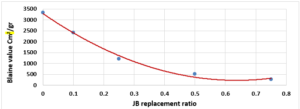
The fineness of the mixture decreases as the JB replacement ratios increase as shown in (Figure 1). The mixture’s fineness affects the workability, durability, strength, and hydration rate. This decrease is due to the increase in JB related to cement because it is finer than JB which was produced manually.
properties of fresh paste and mortar:
Study of Initial and Final Setting Times of Cement-JB vs. JB Replacement:
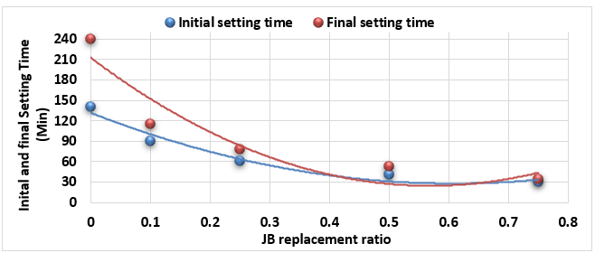
Figure 2 illustrates the relationship between the initial setting time and final setting time (measured according to ASTM C-191) of the mixture of cement-JB pastes with the JB replacement ratios.
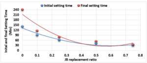
In the analysis of Figure 2, it can be noted how the initial and final setting times of the cement-JB mixture pastes decreased by increasing JB replacement ratios. At the 50% and 75% JB of the mixture, the initial and final setting times are close to each other. The decrease in both initial and final setting times of mixtures is due to the increase in JB, which causes them to lose their elasticity and become sufficiently rigid.
Study of Expansion of Cement-JB vs. JB Replacement according to Le Chatelier:
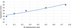
The expansion value of the cement and JB pastes versus JB replacement according to Le Chatelier is shown in Figure 3. The expansion value of the cement-JB mixture mortars increased by the increasing of JB ratios as shown in Figure 3. All of JB ratios do not show any significant expansion values. This increase is due to the fact that JB has a larger percentage of pore voids and is less homogeneous than cement, which was produced manually, and therefore has greater expansion values.
Study of Water Absorption value:
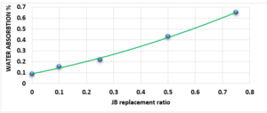
Figure 4 characterizes the water absorption value of cement-JB mixture mortars versus JB replacement, as the increase in the percentage of JB increases the water absorption value. JB is hydrophobic, as the increase in the percentage of JB increases water absorption value (In this case, I think that JB should be hydrophilic rather than hydrophobic). It can be clearly distinguished that all these values are less than 70%. Water absorption is the movement of liquid within unsaturated JB-cement samples’ pores under no external stress. JB, which possesses higher porosity, is known to have a more water absorption capacity, causing an increase in the absorption rate as JB content increases.
Properties of hardened mortar:
Compressive and Flexural Cement-JB Mortar Strength: Compressive and Flexural strength of the cement-JB mortar mixtures were determined at 2, 7, and 28 days of standard curing conditions (20 ± 2°C, and relative humidity >95 or immersed in water) as it is shown in Figures 5 and 6.
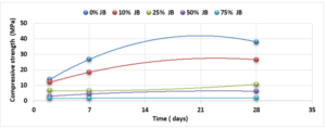
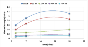
The values of compressive strength cement-JB mixture mortars are shown in Figure 5. The highest compressive strength can be clearly observed in the control samples (38 MPa), followed directly by mixtures containing 10% of JB (26.5 MPa), and then by 25% of JB (10.5 MPa). On the other hand, the lowest compressive strength of cement-JB mixture mortars was obtained at 75% of JB, reaching 1.9 MPa. Adding JB to cement causes an increase in the volume of the mortar, which leads to cracking of the bonds that connect the aggregates, thus reducing the compressive strength. The outcomes derived from the flexural strength tests are shown in Figure 6. This figure displays how the cement mixtures containing 10% of JB have higher flexural strength values than the other three JB ratios investigated (0.86 MPa). When JBs are added to cement, mortar volume expands, breaking bonds and reducing flexural strength.
Study the change of dry density according to the JB replacement ratios: The dry density of the cement-JB mixture mortars with the JB replacement ratios at 28 of curing days are shown in Figure 7.
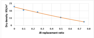
It can be simply detected that increasing the JB ratio decreases the dry density. Reducing density is attributed to certain physical properties, specifically the difference in specific gravity between JB and cement. Additionally, JB exhibits a higher porosity compared to cement, leading to increased volume and reduced overall density.
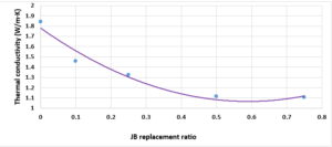
Investigation of the thermal conductivity (K-value) of the replacement of JB:To illustrate the relationship between thethermal conductivity of cement-JB mixture mortars versus JB replacement ratios, the K-value were determined. JB is categorized by low thermal conductivity against the cement mortar as shown in Figure 8, where the thermal conductivity decreases as the JB ratio increases. In general, as the JB content increased, the k-value decreased, because of its heat-insulating properties, as explained previously. The low K-value indicates that JB can be used as a suitable mortar for high-temperature applications.
DISCUSSION
Compared with the ASTM C1329 specification, the mortar cement-JB of 10% of JB can be used instead of type M mortar cement (20 MPa) [17]. While the mortar cement-JB of 25% of JB can be used instead of type S mortar (14.5 MPa), which is used in building parts for exterior, at or below grade, and that of 50% of JB may be used instead of type N mortar (6.2 MPa), which is used in building parts for interior non-load-bearing[17]. According to the ASTM specification, the cement-JB mortar of 10% of JB can only be used as type M mortar (0.8 MPa) [17]. While cement-JB mortars with other ratios of JB cannot be used. The initial setting time at 10% of JB is 90 min, which is in accordance with types S and M (not less than 90 min) According to the ASTM C403 specification. As for the final setting time, not more than 1440 min, all of the final setting times are smaller than this value. These setting times are important factors that affect the strength, durability, and workability of cement. For this reason, 10% of JB can be considered a suitable additive for cement within the standard limit to accomplish the best outcomes in building projects. The maximum expansion ratio at 75% reached 24 mm compared to 0% of JB, which was 16 mm. As for mortar with 10% of JB was 18 mm (only 2 mm increasing related to 0%). Thisconfirms that the JB does not display any considerable consequent expansion. If the expansion value is more than 10 mm, the JB-cement mortar is unreliable as described in ASTM specifications [17]. Consequently, the addition of JB had a positive outcome in the avoidance of the shrinkage property of cement that may lead to the formation of plaster cracks or deficiencies. A higher cement fineness provides very good quality, where smaller particles react faster than bigger particles. A cement particle that has a size of 10µm needs around 30 days to achieve the entire reaction, whereas a particle with a size of 1µm does not need more than 24 hours to achieve the entire reaction [18]. All of the water absorption ratios are less than 70%, which satisfies the conditions of ASTM specifications [17]. Cement mortar needs more amount of water (before and after applying, which causes the site to get very dirty) than the JB containing mortars, which means more time during the curing period in contrast with JB mortars that dry quickly and do not require any more treatment water. Mixing JB with cement at different proportions of 10%, 25%, 50%, and 75% of the cement weight does not considerably modify the dry density of the control cement mortar, which was about 18.9 KN/m3 and for the cement-JB mortar of 10%, 25% of JB was 16.5 and 15.1 KN/m3 respectively, and the reduction ratio relative to the control cement mortar was 14.5 %, 20% respectively. The two preceding types of cement-JB mortars are considered to be heavy-weight (greater than 15 KN/m3) [19]. Consequently, the addition of JB had a positive outcome in the avoidance of substantial volume changes, which lead to cracks in the plaster, or adherence deficiency to the wall support. The quantity of energy needed to cool and heat a building is reliant on the k-value [20]. The materials with a lower value of thermal conductivity have greater capability to restrain heat transmission. There are many factors affecting k-value such as mixture kind, percentage of fine aggregate, total volume of aggregate percentage, ratio of (W/C), humidity and temperature conditions, and additive types (fly ash silica fume, blast furnace slag) [20]. The results show that the thermal conductivity of cement-JB mortars increases as the ratio of JB of it gets larger. Thus such mortars are suitable for high-temperature applications and that is why the ancient residents of Deir EZZOR, whose weather is considered to be very hot, have been using the mortar of pure JB to cover their homes.
CONCLUSIONS
This paper presents the potential of combining JB and cement in the process of production of cement-JB mortars that may be used in the construction sector. Although the obtained compressive and flexural strength values were lower than those of control cement mortar, there is an encouraging outcome of the usage of JB in cement-JB mixture mortars, as the compressive strength at 10% of JB, meets the standard specification for type M cement mortar. Whereas the cement-JB mortar at 25% of JB may be used instead of type S mortar. The addition of JB to the cement mortars decreases the thermal conductivity, which gives good thermal properties and ensures energy saving. Cement mortar is prone to cracking, most cracks are caused by shrinkage, which is very common, while JB-added mortar has high elasticity and is less prone to cracking, All of the JB ratios do not show any significant expansion values, where the maximum ratio of 8 mm compared to 0% of JB. In addition, the JB is hydrophobic which results in the moisture not remaining on the interior walls for a long time which will cause no formation of mould and mildew on these walls and prevent them of being slippery. JB-cement mortar dries quickly, which has a 90 min initial setting time at 10% of JB, so it does not require any additional treatment water as the cement mortar which needs a great amount of it (before and after applying). The study also stated that increasing the JB ratio decreases the dry density; the reduction ratio was 14.5 %, 20% at 10%, 25% of JB, respectively. More particularly, it has been probable to confirm that the cement-JB mixture mortars with 10% or 25% of JB accomplish worthy properties, although these mortars do not meet the standards achieved by control cement mortars. On the other hand, the cement-JB mixture mortars may be used in rehabilitation works and rural buildings as a sustainable solution. Also, they can be used, as they were locally used, as interior coverage of walls and roofs in high-temperature cities like Deir EZZOR to reduce their thermal conductivity and make houses more thermally comfortable.

Journal:![]() Syrian Journal for Science and Innovation
Syrian Journal for Science and Innovation
Abbreviation: SJSI
Publisher: Higher Commission for Scientific Research
Address of Publisher: Syria – Damascus – Seven Square
ISSN – Online: 2959-8591
Publishing Frequency: Quartal
Launched Year: 2023
This journal is licensed under a: Creative Commons Attribution 4.0 International License.