قسم : Research Articles

Preparation of Nanosilica and Nanosilicone from Glass Wastes
Modeling Volume, Basal Area and Tree Density in the Kalala Forest in Northern Iran Using Sentinel-2 Satellite Data and Random Forest Algorithm
A D-Metric Analysis of the Denomination Structure of the Syrian Pound
INTRODUCTION
Although coins and banknotes are in issues for decades, there is no agreement amongst economists on what is the theoretically optimal denomination structure of a currency [1]. Two components are usually used to identify any denomination structure, those being the structure boundary and the series within the boundary. The structure boundary includes determining the lowest coin value, the highest banknote value and the transition between coins and banknotes. The series inside the boundary includes the number of coins, banknotes, and total number of denominations [2]. Determining the optimal denomination structure of a currency is a daunting task. It involves ensuring the efficiency of the structure, its cost effectiveness and its balance in terms of having a proper mix of the various denominations [3] [4]. To ensure this task is well handled, central banks need to closely monitor the evolving changes (technology, security issues, high inflation..etc) and timely respond to them [5]. Empirically, [6] proposed the D-Metric model to determine the denomination structure of the currency. The model utilizes the relationship between the average daily wage level (D) and the denominations of the currency to identify the coins on the lower scale that need to be withdrawn from circulation, the boundary point between coins and banknotes, and the appropriate timing for the introduction of higher banknotes [7]. This study uses the D-Metric model to analyze changes in the denomination structure of the Syrian Pound between 1997 and 2022. The choice of the period is to capture the last three changes in terms of introducing a higher banknote in Syria. The study was motivated by the scarcity of previous research on the optimal denomination structure in general and in Syria, in particular. The study was further motivated by the public attention that accompanied the introduction of the SP5000 and the rumors regarding the potential issuance of the SP10000. The aim of this study is twofold. First, to analyze the denomination structure of the Syrian Pound and to verify whether the introduction of the last three high denomination banknotes was justified from the D-Metric model point of view. Second, to analyze whether a higher banknote should be introduced. The study contributes to the literature on the optimal denomination structure as it is the first that analyzes the denomination structure of the Syrian currency using the D-Metric model. The findings of the study have empirical implications for the Central Bank and the public in Syria. They will enable recommending the denomination of the higher banknote that should be issued and the timing of this issuance. The remainder of the study is organized as follows: Section one sheds light on the currency structure in Syria. Section two explains the D-Metric model. Section three analyzes the denomination structure in Syria using the D-Metric model. Section four concludes the paper.
The Currency Structure in Syria
The monetary authorities and denomination structure in Syria passed through several historical landmarks. Below is a brief highlight of this main historical changes. In the era of the French Mandate, the Bank of Syria supervised the process of issuing the currency. The name of the bank changed later on during that period to become the Bank of Syria and Lebanon. After gaining independence, the Bank of Syria and Lebanon continued on issuing the currency in both Syria and Lebanon. However, it was replaced later on by the Syrian Institute for Issuing Money. In 1953 the Legislative Decree No. /87/ was issued [8]. The Decree defined the basic monetary system in Syria and established a Council for Money and Credit to take on the tasks of the Central bank. The Central Bank of Syria did not officially start working until 1/8/1956. Below is a review of the development of the currency structure since the Central Bank of Syria became responsible for supervising the issuance of the Syrian Pound, the official currency in the Syrian Arab Republic. Figures (1) and (2) below show the development of the currency structure after the Central Bank of Syria became responsible for issuing the Pound. As per the structure of coins, after its establishment, the Central Bank of Syria continued to issue coins in the denominations of 2, 5, 25 and 50 Piasters and one Pound that previously existed. In 1960, a new coin in the denomination of 10 Piasters was issued for the first time. As shown in Figure (1), the structure of the coins remained unchanged until 1995, when new coins in the denomination of 25 Pounds were issued. In 1996, new coins in the denominations of 2, 5 and 10 Pounds were issued for the first time. In the same year, coins in the denominations of 2, 5 and 10 Piasters were withdrawn from circulation. In 2004, coins in the denominations of 25 and 50 Piasters were withdrawn from circulation. At the end of 2018, the highest denomination of coins, 50 Pounds, was issued [9]. With regard to the structure of banknotes, the Central Bank of Syria continued to issue banknotes in the denominations of 1, 5, 10, 25, 50 and 100 Pounds which previously existed. In 1958 a new banknote in the denomination of SP500 was issued for the first time. As Figure (2) reveals, the structure of banknotes remained unchanged until year 1997, when banknotes in the denominations of SP200 and SP1000 were issued for the first time. More than ten years in the Syrian crisis, which started in 2011, caused a massive economic destruction to the Syrian economy. The Syrian Pound which had a pre-crisis exchange rate on the average of USD1= SP45 gradually depreciated to exceed USD1= SP3800 in the black market. The depreciation of the Syrian Pound and the high inflation that Syria was facing triggered many questions regarding the necessity of issuing higher banknotes. In 2015, with the annual inflation rate reaching an average of 38.46%, the SP2000 note was printed for the first time. It was put into circulation in July 2017 when the annual inflation rate was 14.48% [10]. Recently, in 2021, a new note in the denomination of SP5000 was put into circulation. The 5000 note was printed in 2019 when the annual inflation rate was, on average, 13.42%] [10]. According to the official releases of the Central Bank of Syria, the SP5000 note was printed to meet the trading needs of the public in a manner that ensures facilitation of monetary transactions and reduces the cost and intensity of dealing in banknotes. The Central Bank reported that the current economic changes, and the significant rise in prices that started in the last quarter of 2019 and continued during 2020, made the timing appropriate for putting the SP5000 into circulation [10]. Following the issuance of the SP5000, there was a public debate on whether the SP10000 needs to be issued and put into circulation or whether it is premature to do so.
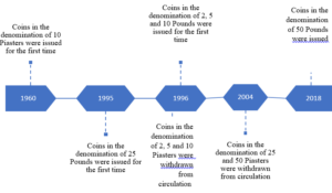 Figure (1): Timeline of the development of the coin structure in Syria
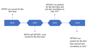
Figure (2): Timeline of the development of the banknote structure in Syria
The following section introduces the D-Metric model that will be used to analyze the changes in the currency structure in Syria since the introduction of the three highest banknotes (SP1000, SP2000, and SP5000).
MATERIALS AND METHODS
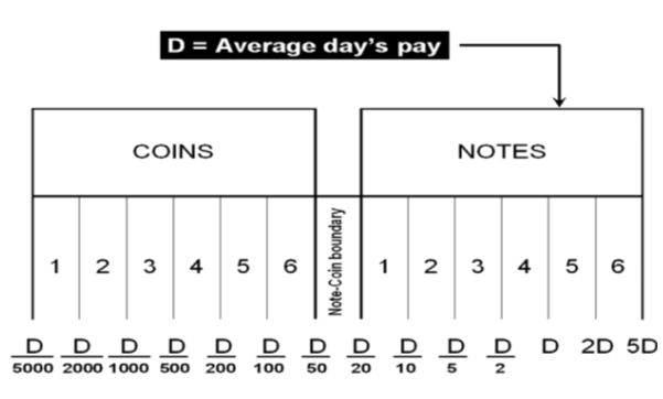
The D-Metric model
Determining the optimal denomination structure includes identifying the structure boundary and the series within the boundary. That is to say, identifying the lowest coin value, the highest banknote value and the transition between coins and banknotes along with the number of coins, banknotes, and total number of denominations inside the boundary. The spacing of the denominations in most countries is based on either a binary-decimal triplets system (1-2-5) or a fractional-decimal triplets system (1-2.5-5) [2]. Syria is amongst countries that adopted a mix of the two systems. It has six denominations of coins (1, 2, 5, 10, 25, and 50) and seven denominations of banknotes (50, 100, 200, 500, 1000, 2000, 5000). The denomination of (5, 10, and 25) banknotes are legal tender although they are not issued any more by the Central Bank. As can be seen, the denominations (10, 25 and 50) follow the (1-2.5-5) system while the rest of the denominations follow the (1-2-5) system. Trying to figure out the optimal denomination structure, [6] used data from sixty currency-issuing authorities around the world. They documented a consistent relationship between the average daily pay (D) in a country and its currency structure. They reported that in most of the examined countries, the boundary denomination between coins and banknotes is located between D/50 and D/20. The top and lowest denominations are around five folds of the average daily pay (5D) and 5000 parts of the average daily pay (D/5000), respectively [12]. As shown in Figure (3), the model assumes that there are six denominations of coins and six denominations of banknotes along with one denomination at the boundary between coins and banknotes. The model can be used to advise when a modification on the denomination structure is needed. This includes the modification of the lowest-highest denominations and the transition between coins and banknotes [2]. The D-Metric model, however, is subject to several limitations. First, it is a practical method that lacks a theoretical base. Second, it ignores other factors that should be taken into consideration when determining the denomination structure of a currency. This includes, the costs associated with economic agents and users’ preferences, including payment habits [13] [14] [15]. The model also ignores the fact that payment habits, culture and wealth holding might differ across countries and could vary, within the same country, over time. In addition, the model fails to take into account the durability of monetary items and their costs when determining the boundary point between coins and notes [2]. Despite being subject to several limitations, the simplicity of the D-Metric model makes it used as a guideline to the re-denomination of currencies and it has been successfully applied in a wide range of countries around the globe [12] [16] [17]. The following section will utilize the D-Metric model to analyze the denomination structure in Syria between 1997-2022.

RESULTS
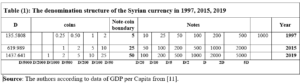
As Figure (2) indicated, bigger banknotes were issued in 1958, 1997, 2015 and 2019. Our analysis of the denomination structure in Syria is limited to years 1997, 2015 and 2019. Year 1997 was chosen as it experienced the last issuance of a higher banknote, the SP1000, prior to the eruption of the Syrian crisis.[1] Years 2015 and 2019 were chosen as they are the years in which the two higher banknotes, the SP2000 and SP5000, were issued. Years between 1997 and 2015 were not examined as there are no issuance of higher banknotes in these years. As highlighted earlier, the D-Metric model relates the average daily wage level to the denomination structure of the currency. Due to data availability issues, the nominal GDP per capita per day was used as a proxy for the average daily pay (D in the D-Metric diagram). The daily GDP per capita was adopted by many authors on their application of the D-Metric model [2] [12]. Table (1) reveals the value of D and the denomination structure in each of the examined years.
DISCUSSION
Starting with year 1997, the D-Metric model suggests that the lowest useful coin should be between SP0.02 (D/5000) and SP0.067 (D/2000). The note-coin boundary should be between SP2.7 (D/50) and SP6.7 (D/20), suggesting that the higher coin should be SP5, which can be either a coin or a banknote. The largest banknote suggested by the model is the SP500 banknote which falls between SP271 (2D) and SP677 (5D). Table (1), however, reveals mismatches between the theoretical denomination structure suggested by the D-Metric model and the actual structure in year 1997. To be more specific, the lowest coin, 25 Piasters (SP0.25), lies between D/1000 and D/500 instead of D/5000 and D/2000, as suggested by the model, and the highest coin is SP25 instead of SP5.[2] In addition, the SP10 and SP25 exist in coins and banknotes whereas the model predicts that the note-coin boundary should be SP5. Another mismatch with the D-Metric model is the existence of the SP1000 banknote whereas, according to the model, the highest banknote should be SP500 (between 271 and 677.9). Accordingly, based on the D-Metric analysis of the currency structure in year 1997, one can conclude that the structure is not the optimal one and that the introduction of the SP1000 was premature and should have been postponed until year 2005 when 5D was equal to SP1124.219. The structure recommended by the D-Metric model changes in 2015 in comparison to that in 1997. As shown in Table (1), the SP25 got pushed into the note-coin boundary whereas the SP5 and the SP10 fell into the coin category. Furthermore, the SP2000 banknote became the largest useful banknote. Unlike the mismatch in year 1997, it seems that the currency structure in 2015 complies with the theoretical denomination structure suggested by the D-Metric model in this year. The highest coin in circulation in 2015, SP25, falls into the note-coin boundary (D/20=619.989/20=30.999) and (D/50=619.989/50=12.399) and the highest banknote, SP2000, falls between (2D=2*619.989=1239.978) and (5D=5*619.989=3099.945). Therefore, it was appropriate, then, to issue the SP2000 banknote in this year. In fact, it was even appropriate to issue it in 2014, when D was SP471.6 (2D=943 and 5D=2358) [11]. Since the SP2000 was printed in 2015 but not put into circulation until 2017, the analysis requires examining whether it was put into circulation on the right timing. Knowing that in year 2017, D was equal to SP1053.99, the SP2000 falls outside what is suggested by the model (2D=2107.98 and 5D=5269.95). Accordingly, the delay in introducing the SP2000 into the market was inconsistent with the denomination structure suggested by the D-Metric model. In fact, the D-Metric analysis suggests that the SP5000 banknote could have been put into circulation in 2017 and not just the SP2000. As can be seen from Table (1) the structure recommended by the D-Metric model changes in 2019 in comparison to that in 2015. The SP50 got pushed into the note-coin boundary whereby the SP25 fell into the coin category. Furthermore, the SP5000 banknote became the largest useful banknote (lying between 2D=1437.641*2=2875.28 and 5D=1437.641*5=7188.2). The Table also reveals that the lowest useful coins for this year, SP1 and SP2, fall within D/2000-D/1000 and D/1000-D/500, respectively. The lowest useful banknote, SP50, falls into the note-coin boundary (between (D/50=1437.641/50=28.75) and (D/20=1437.641/20=71.88)). This means that the decision to issue the SP50 coin was appropriate. Adhering to the 1-2-5 system of spacing, the next useful banknotes would be 100, 200, 500, 1000, 2000, 5000 according to the model. Indeed, those are the currencies that are actually in circulation in that year. Although it is justified to put the SP5000 banknote in circulation since 2017 as indicated above, the note was not put in circulation until 2021.
Should a higher banknote be put into circulation?
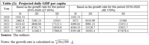
Recently, there are discussions among the public and economists regarding the necessity of issuing a higher banknote (the SP10000 banknote). Issuing higher banknotes has its own advantages and disadvantages. One of the main advantages is the easy handling of transactions as people do not have to carry large quantities of money to do their daily transactions [20]. This is especially important bearing in mind the high reliance on cash and the very low reliance on E payment in Syria. Another advantage is the lower carrying and management expenses, as according to the Central Bank of Korea, issuing the higher denomination allowed a saving of 60 billion won (approximately USD 50,000,000) every year due to reductions in management expenses especially those related to logistic costs [21]. In addition, the higher notes have lower production costs as they are less frequently used and used with more caution than is the case for smaller notes [13]. The higher notes could also help reduce spending as people are less encouraged to buy something if they have to pay one big note than is the case if they are paying with several smaller notes [13]. Issuing higher notes might also protect the national identity of the country by reducing the chances of substituting the domestic currency for other currencies (dollarization) [22]. The major disadvantage of issuing higher banknotes, lies on the inflationary impact of issuing higher notes, which could be a very serious one. As expectations of inflation drive up inflation, the higher note might be followed by higher inflation. The fear is that if the cycle starts, it is not easy to stop it. More precisely, if inflation increases after the issuance of the higher banknote, this might lead to the issuance of a higher note and the cycle goes on. Other disadvantages of issuing a higher note revolves around production costs, susceptibility to forgery and facilitation of drag dealing and illegal activities [23] [24]. To determine whether a higher note, the SP10000, should be issued, we applied the D-Metric model on the daily GDP per capita for the year 2020 where D is equal to SP2101.06 [11]. As highlighted earlier, according to the model the highest note should be between 2D and 5D. This means that the highest note should be between SP 4202.12 and SP10505.3. Accordingly, the D-Metric model suggests that the SP10000 could have been issued and put into circulation since 2020. The high inflation that Syria is still facing makes us in doubts of whether a higher banknote should be issued as the SP10000 might not be enough to meet the needs of the daily transactions. Table (2) reveals the results of applying the D-Metric model on the daily GDP per capita for the year 2021 where D is equal to SP3099.93 [11]. As the table reveals the 2D and 5D are 6199.86 and 15499.65 respectively. This indicates that the 10000 note is enough and no higher note needed to be issued in that year. Unfortunately, no data of the daily GDP per capita for the year 2022 is available to conduct the analysis. To circumvent this issue, we tried to extrapolate the expected growth rate based on the historical growth rate, under two scenarios. In the first scenario, we used the daily GDP per capita in years 2015 and 2021 to calculate the average growth rate for the period.[1] This was then used to project the future daily GDP per capita on the following years. In the second scenario, we assumed that the growth rate on the daily GDP per capita between years 2020 and 2021 would remain unchanged, and we used this growth rate to project the future daily GDP per capita on the following years. Table (2) reveals the results of applying the D-Metric model based on both of the simulated scenarios. As Table (2) reveals, applying the average growth rate for the period 2015-2021 shows that the issuance of the SP20000 could be done in 2023 and should not be pushed beyond 2024. However, applying the aggressive growth rate, the one that is based on the growth rate of years 2020-2021, reveals that the issuance of the SP20000 could be done in 2022 and should not be pushed beyond 2023. The fact that the SP10000 could have been issued and put into circulation since year 2020 and that the SP20000 should not be pushed beyond 2023-2024, indicates that the monetary authorities might have to issue both of the banknotes, 10000 and 20000, at one time or within a short time span. This, however, might have adverse outcomes on the inflation levels that are already high!
CONCLUSION AND RECOMMENDATIONS:
The aim of this study was to analyze the denomination structure of the Syrian Pound between 1997 and 2022 and to examine whether the decisions of issuing the higher banknotes (SP1000, SP2000 and SP5000) were justified based on the D-Metric model predictions. The study also aimed to examine whether higher banknotes (SP10000 and SP 20000) need to be issued and put in circulation and what is the appropriate timing for this. The study was mainly motivated by the recent issuance of higher banknotes in Syria along with expectations of further issuance of higher banknotes. When comparing the denomination structure in the examined period with that suggested by the D-Metric model, the findings revealed that the introduction of the higher note, SP1000, in 1997 was premature and should have been postponed to 2005, however the issuance of the SP2000 was on the right timing. The delay however in putting the SP2000 in circulation was not consistent with the outcomes of the D-Metric model. The SP2000 was put into circulation in 2017 when it was appropriate to issue the SP5000. The findings also reveal that the issuance of the SP5000 in 2019 was consistent with the predictions of the D-Metric model. When examining whether a higher banknote, SP10000, should be issued, the D-Metric model suggests that the SP10000 could have been issued and put into circulation since 2020. The high inflation that Syria is facing now tempted us to examine whether the SP20000 should be issued. To overcome the lack of data on daily GDP per capita after 2021, we used two growth scenarios to simulate the daily GDP per capita for the coming years. The findings indicate that the SP20,000 should not be pushed beyond 2023-2024 the latest. The fact that the issuance of the SP20000 should not be pushed beyond 2023-2024 and that the SP10000 could have been issued and put into circulation since 2020 means that the monetary authorities should not delay the issuance of the SP10000 anymore. Otherwise, the monetary authorities might have to issue the two notes SP10000 and SP20000 at the same timing or within a very short time span. This, however, might have detrimental impact on the public confidence in the currency and might trigger higher and higher levels of inflation. Although the analysis was based on the simple and easy to apply D-Metric model, the popularity of the model among central banks and the cross-country empirical evidence that supported its predictions, allow us to utilize it. The findings obtained when applying the model have important implications to the monetary authorities in Syria. They, the findings, indicate that delaying the issuance of a higher note creates further problems in terms of having to issue a further higher banknote soon, which increases the uncertainty in the market and could create higher inflationary expectations. The findings are also of high importance to the public as finding the optimal currency structure enhances the efficiency of cash payment’s settlement. Despite the important findings of the current study, they should be interpreted with caution due to several reasons. First, as highlighted earlier, the D-metric model relates the average daily pay in an economy and the currency denomination structure, however, it does not take into account other factors that affect the denomination structure. This includes amongst other things, the cost structure and economies of scale associated with the printing and minting of a currency, the presence of extra demand on specific denominations, laws and regulations, public’s perception of inflation, etc. The currency denomination structure of a country is also a function of its past economic and political events which is not taken into account by the D-Metric model [12]. Two areas for future research emerge from this study. First, a multidimensional study that takes into account other factors that could affect the denomination structure is needed to get a better understanding of the suitability of the current and future denomination structures. Second, as issuing higher notes could be a response to the higher levels of inflation, the bidirectional relationship between issuing higher notes and inflation would be very informative to the monetary authorities and the public as very little evidence exists on this area.
A Comparison of Four Information Diffusion Inspired-Based Models According to Real Data Diffusion Similarity
INTRODUCTION
social networks play a crucial role in the dissemination of information. Social media has changed the way people interact with the news. In the past, people only received news and events, while, on the contrary, social networks transformed people into engaged parties by allowing them to create, alter, and spread the news. Currently, many models have been developed to study information dissemination over social networks. The importance of social media in affecting societies has also been considered. The absence of censorship [1] existing in traditional media (magazines and newspapers), makes them promising environment for viral marketing [2], rumor breeding [3], and crowd control by changing their attitudes, brains, and practices. The contribution of this study is the comparison of four new inspired-based models in terms of their similarity with real data diffusion. We focus on this similarity factor because of its importance in social networks. As networks simultaneously reach billions of connected users, the model must comply with good real-data diffusion criteria to be applicable in real-life cases. This paper is organized as follows: In the next section, we discuss elementary diffusion models and some important definitions, and then introduce the four inspired-based models in more detail to show their capabilities. Next, we present and compare the experimental dataset used to test these models. Finally, we discuss the findings and suggest future work. Our research tries to answer the following question: in terms of performance of the four information diffusion models, which one is the most suited for real data diffusion? This aim reflects the goals of the study in comparing different information diffusion models and assessing their performance against real data, which can be valuable for both academic research and practical applications.
MATERIALS AND METHODS
Elementary Models and Definitions
In this section, we discuss the basic models of diffusion and the basic terms used in the remainder of this study. Social networks [4] are intended to disseminate innovations. Kempe et al. [5] are the first who model Influence Maximization (IM) through social networks. In this study, Kempe presented an analysis framework that is meant to be the first approximation guarantee for an efficient algorithm to select the most influential node-set. This framework uses the nature of greedy algorithm strategies to obtain a solution that is 63% suitable for the most basic models. Influence maximization [4] could be defined by selecting a seed set of nodes where the network reaches the maximum influence according to this set. The target of any influence model is to maximize influence and predict how information dissemination paths can be obtained.
Models Representations
A diffusion model represents the social network as a graph G = (V, E), where G is the graph or network, V represents the vertices that model the users in the networks, and E contains the edges that represent the relation or interaction between users in the corresponding social networks. Many diffusion models have been proposed to mimic information dissemination. Li et al. [6] categorized the models into two categories: progressive diffusion models and non-progressive models. In Progressive diffusion models, nodes that are activated or infected by other nodes cannot be recovered or deactivated from the dissemination propagation. Linear Threshold (LT) and Independent Cascade (IC) are examples of these models. Linear Threshold (LT) and Independent Cascade (IC) models are the primary models. LT [7] is defined by Granovetter as a node that can be in one of two states (active/inactive) and can be turned from active to inactive based on the activation function, which is the sum of the weights of the neighbor nodes. If the sum exceeds the threshold, then the node turns on active and starts the diffusion process. If the node is not activated on the first attempt, it will remain inactive on the next attempt. The IC model [8] is more likely to be LT, but the activation function is based on statistical probability to determine whether the node will be active when propagation starts or whether it will remain inactive. In non-progressive diffusion models, the node might be deactivated after some time of activation and stop propagating the diffusion. Examples of non-progressive diffusion models are typical epidemic disease models like the Voter model [6] and the Susceptible-Infected (SI) model [9] and their ancestor’s models Susceptible-Infected-Susceptible (SIS) [9] and Susceptible-Infected-Recovered (SIR). Kermack at al. proposed the Susceptible-Infected-Recovery (SIR) model [10], which is an epidemical model that considers the population as constant, while the nodes could fall into one of three modes: Susceptible where the node can get infected by the disease, Infected where the node is infected by the disease and Recovered where the node has recovered from the disease and will not get infected again. The basic models mentioned above were used in all proposed models.
Related Works
Experiments conducted with actual real-world data have played a crucial role in evaluating the effectiveness and practicality of diffusion models. These investigations highlight the importance of testing models under lifelike conditions, offering valuable insights into the intricate nature of information spread across different situations. Several noteworthy contributions that have enhanced our comprehension in this regard encompass: Ugander et al. [11] in their influential study, examined the diffusion of information within the Facebook network. By analyzing the spread of content such as news articles and videos, they compared the observed diffusion patterns with predictions from various models. This work revealed the nuances of information flow within an online social network, shedding light on the models’ capabilities and limitations in capturing real-world dynamics. Myers et al. [12] explored the retweeting behavior on Twitter, focusing on how information spreads through the network. By investigating the viral diffusion of tweets and memes, they provided insights into the role of influential users and the temporal dynamics of retweets. This study highlighted the need for temporal considerations in diffusion models and emphasized the significance of early adopters. González-Bailón et al. [13] Investigating the diffusion of content across the blogosphere, he examined the interplay between the content’s virality and the network structure. They found that diverse and well-connected blogs are more likely to spread information widely. This study showcased how the characteristics of the dissemination platform interact with the content itself to influence diffusion patterns. Bakshy et al. [14] studied the diffusion of news articles on Facebook, revealing the role of social influence and algorithmic curation in shaping the visibility and spread of content. They found that exposure to friends’ interactions with news stories significantly influenced users’ engagement. This work highlighted the interplay between social connections and platform algorithms in information diffusion. Weng et al. [15] conducted a comprehensive comparison of different information diffusion models using Twitter data. By analyzing the spread of hashtags, they evaluated the performance of models like Independent Cascade and Linear Threshold in predicting real-world diffusion. This study contributed to the understanding of how different models approximate observed diffusion patterns. Building upon the traditional models, Liu et al. [16] introduced a dynamic variation, the Time-Critical Diffusion Model, which incorporated temporal factors for predicting information spread. Their work highlighted the temporal aspect as a crucial component of diffusion modeling, especially in scenarios where the urgency and timing of information propagation play a critical role. Smith et al. [17] conducted an empirical study comparing several diffusion models on real-world social network data. Their findings revealed that the performance of models varied significantly depending on the characteristics of the network and the nature of the information being propagated. Additionally, Kumar et al. [18] introduced a new model called the modified forest fire model (MFF). Their work is based on the enhancement of an existing model and the introduction of the term ‘burnt’ to represent nodes that stop propagating information. They used real Twitter datasets to compare their model with the SIR and IC basic models to demonstrate the feasibility of their work.
Theory/Calculation
Many studies have focused on models inspired [1, 19-21] by physics, sociology, mathematics, and so on. In addition, optimizations can be obtained from these inspiration-based models to solve complex computational issues using swarm-based intelligence or to mimic natural phenomena to solve optimization problems.
Diffusion Models
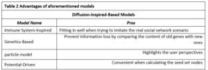
In this study, we focus on four different inspired-based models to demonstrate their ability and the limitations that need to be addressed in future research. These models were selected based on their popularity and the publication dates of their research. Similarity to the diffusion of real data appears to be the most important comparison feature when dealing with social networks. Predicting the diffusion paths of any post or tweet can help in predicting its consequences and effects, the data provenance of rumors after rumor diffusion, or sources of fake news. Table 1 provides a short description of each of the four models.

Immune System-Inspired Information Diffusion Model
The Immune System-Inspired information diffusion model proposed by Liu et al. [21], mimics the immune system of the human body. The human immune system attempts to handle and eliminate non-self-material by recognizing microbes and studying their information to decide the best way to deal with them. However, immunity deals with antigens in different ways, using memory to prepare for action, either leaving or trying to eliminate them. This biological structure of immunity resembles the information diffusion process, where antigens represent the information received by users, and antibodies represent the users who receive the information. User responses to information vary from one user to another according to their immune system, which is represented by the fitness function. The fitness function could be formulated according to Liu [21] as

Where and represents the neighbors of node I and j in time t, when the information is disseminated, respectively. The equation represents the common friends of the node and at time . represents the degree of an entire network while the is the degree of node . and are weighted variables determined by the network structure. The calculation of the fitness function determines whether the value exceeds the activation threshold to start diffusion or is below the threshold to keep the information on the immune list, where it will be ignored. The immune list retains this information as a long-lasting memory to keep discarding it when the body receives it again. Diffusion between persons is not constant, as in other non-inspired models, but it is a dynamic diffusion that varies from one person to another. One of the greatest limitations of this model is that it considers time. Time progress increases the immunity of the nodes and decreases the diffusion process. In addition, this model assumes that all the nodes are simultaneously active, which is not the case in reality. Moreover, this model does not consider the content of the information, which is a critical aspect of diffusion. Different information expressions lead to different diffusion paths. However, this was not considered in the model. This model must find the most influential node with a high degree of connection to accelerate diffusion. The saturation of diffusion of a single node leads this node to lower its immunity and propagate the information forward.
Genetics-Based Diffusion Model
The Genetics-Based diffusion model was proposed by Li et al. [20]. The idea behind this model is to use a genetic algorithm (GA) to mimic the diffusion process in social networks. The chromosomes represent the nodes, and the gene represents the message. This model was built on top of the epidemic-spread susceptible-infection model. The main objective of this model is to spread multiple objects with different relationships across various social media platforms despite the other spreading models. The process of this model starts with crossover when the genetic algorithm begins, and the new gene contains the information that will spread across the network. The cross-over may lead to a split of the information which is called information loss. However, this problem is solved by comparing the content of the old genes with that of the new ones to ensure that the information is preserved. The breakpoint is the term meaning that the spread starts slowly until it reaches this point; then, the spread starts increasing rapidly. The computational cost [12] of this algorithm is low, because it’s depending on the directed graph where information is passed from the sender to recipients. This imposes to take action if the diffusion must be stopped before reaching this point. A weakness of the proposed model appears when only one message that spreads the information behaves exactly like the way in the Susceptible-infected (SI) model; the model failure appears [12] when attempting to spread two contradictory pieces of information as the experiment done by Li, which ends with slowing propagation and making its result unpredictable. The experiment yielded different results when conducted using two independent messages. Therefore, the behavior of this model did not proceed as expected. The best performance appears with dependent information.
Particle-Model of Diffusion
The particle model is inspired by the elastic and inelastic collisions of particles. It is presented by Xia et al. [1]. It is based on the particle collision system, where the influence of diffusion is represented by the kinetic energy obtained from the particle collisions, while the user influence is represented by the particle mass. Xia represents this model on a smooth surface to represent the particle collisions on the damping orbit. He [1] formulated a model as follows: the user should be considered a mass particle. After a collision in orbit, the user can be in one of three states:

Where: represents the energy particle k obtained from after the collision. represents the energy particle k needs to pass the damping track. When the particle has the energy to pass through the damping orbit, it hits other particles and spreads information. The particle stops at the damping track when it has no energy to continue colliding with other particles, so the particle will be in a contracting state. Otherwise, the particle will never collide with the other particles, which represents the user in the inactive mode. The primary feature of this model is to highlight the user’s perspective in information diffusion, where the user’s influence plays a crucial role in the process. This model is based on the Susceptible-infected (SI) model. This model can work with a big network according to the proposed article where he could deal with millions of spreaders and larger networks [1]. The weakness of this model is that it varies depending on the initial set that determines its ability to diffuse. Diffusion starts slowly and then grows rapidly with time, and collision continues.
Potential-Driven Diffusion Model
The last model is the Potential-Driven Model, it is proposed by Felfli et al. [19]. This model takes advantage of a physically inspired approach. The nodes were represented as particles. The relationship between nodes is represented by the forces between particles. Each particle creates a potential at its location, which determines the influence of forces between nodes in the graph. The proposed architecture can yield good results compared with greedy algorithms, which are used to calculate the seed set to achieve influence maximization (IM) in the network; however, the computational cost of calculating this set is high, to determine the potentials for individual nodes, the net potential algorithm exhibits [19] a computational complexity of O(n2), where n represents the network’s size, specifically the number of nodes it comprises. The most resource-intensive step within this process is the calculation of pairwise distances (RSP), as it necessitates the inversion of an n x n square matrix, giving rise to a computational complexity of O(n3), which limits this approach to small networks and makes it infeasible for large networks. The researcher limits the samples of their networks during the experiments to be varying from 250 to 100,000 nodes, because of its highly computational cost. In addition, the features of timestamp, location, topic, and feel add complexity to the selection of seed nodes. This model [19] attempts to use the simulation-based approach or the sketch-based approach. The simulation-based approach variation is based on a greedy algorithm and Monte Carlo simulation. The sketch-based approach avoids using the extensive Monte Carlo calculation by using grounded sketches under the dissemination model. The most important feature of the potential-driven model is its ability to mimic the influence between nodes, such as forces between nodes. It uses an approximation to calculate the influence score of the entire network by considering this network as a closed static system of particles. This model is considered an extension of the linear threshold model. Static networks are considered one of the biggest limitations of this model. Tables (2 and 3) presents consecutively the pros and cons of the models mentioned above.
Experiment:
Selecting the diffusion model to be used in any case depends on several factors. These factors vary depending on the model’s capabilities for adapting to large networks, dynamic networks, and similarity to real data diffusion paths. The resemblance between the selected model and real diffusion offers a great opportunity for responsible parties to predict the results and consequences of the diffusion of any posted information on society.

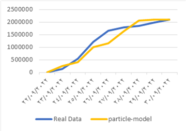
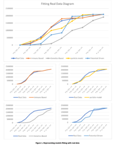
In fake news spreading, the model provides the ability to trace the information after starting the diffusion to locate the false news spreader and take appropriate action to stop the dissemination. We applied the previously listed models to determine which one best fit the real data. We selected a hot topic that has recently arisen, “death of people after boat sinks off”. This information first appeared on Thursday September 22, 2022. We collected 2.1 million blogs from 22nd September to 30th September, then we counted the users who discussed this topic. The data collected using the twitter API development by selecting the trends and collected the users and data. The data collected by help from https://www.kaggle.com where the researchers could ask them to collect a data-set. Furthermore, we utilized a data-set sourced from the Twitter social network [22], specifically related to the hashtag #Bitcoin. Bitcoin, a decentralized digital currency commonly known as a cryptocurrency, was introduced in 2009 by an individual or group using the pseudonym Satoshi Nakamoto. The dataset encompasses tweets extracted from the period of January 21, 2021, to May 31, 2022, comprising approximately 4,569,721 tweets. In the experiment, we used the set of users who first posted the information on the first day as a seed set (initial value for node activation), and we implemented the four previous models on this data to find the best model for both data-set. The x-axis represents time, and the y-axis represents the number of engaged users in the dissemination of information over time. The similarity of the previous model with real data is shown in Fig.1. and Fig.2.
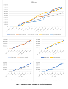
RESULTS
The findings of our research paper shed light on the performance and effectiveness of four different diffusion models: the Genetic-based Model, Potential-driven Model, Particle Model, and the Immune-based Model. Each model was subjected to rigorous experimentation and evaluation against real-world diffusion data to understand their strengths and limitations in accurately representing information dissemination dynamics in networks.
EXPERIMENT METHODOLOGY
- Selection of Diffusion Models: We selected four different diffusion models, each presumably designed to represent the spread of information in networks in a unique way. These models are the Genetic-based Model, Potential-driven Model, Particle Model, and the Immune-based Model.
- Collection and Analysis of Real-world Diffusion Data: we collected real-world diffusion data, which likely includes data on how information (death of people) or trends (Bitcoin) spread through networks. This data serves as the basis for evaluating the performance of the diffusion models.
- Data Preparation: The real-world diffusion data was likely cleaned and prepared for analysis to ensure its accuracy and relevance.
- Model Implementation: Each of the four diffusion models was implemented or simulated based on their respective algorithms and methodologies.
- Comparison and Evaluation: The performance of each model was evaluated by comparing its predictions or simulations with the actual diffusion data.
- Strengths and Limitations Assessment: As part of the evaluation, our aim was to understand the strengths and limitations of each diffusion model. This would involve identifying where each model excelled and where it fell short in accurately representing the dynamics of information dissemination.
DISCUSSIONS
Genetic-based Model: The Genetic-based Model exhibits a slow diffusion process initially, characterized by a gradual increase in the spread of information. However, it undergoes a turning point where the diffusion rate rapidly accelerates, leading to a swift dissemination of information throughout the network. While this high rhythm in the later stages might seem promising, it fails to align well with the actual diffusion data. The model’s behavior deviates significantly from the observed real-world diffusion patterns, making it less suitable for capturing the intricacies of information propagation in networks. This model suffers from the overfitting, when the model is trained, it learns to fit the training data as closely as possible, aiming to minimize errors and discrepancies between the model’s predictions and the actual data points. However, overfitting occurs when the model becomes too specialized in capturing the noise and intricacies present in the training data, rather than learning the underlying patterns or relationships.
Potential-driven Model: In contrast to the Genetic-based Model, the Potential-driven Model does not fit well with the real diffusion process at the outset. In the early stages of diffusion, the model exhibits discrepancies with the actual data, indicating its limited accuracy in capturing the initial spread of information. However, as the diffusion progresses towards its final stages, the Potential-driven Model starts to converge and better matches the real data. This suggests that the model’s performance improves in the later stages of diffusion, but it may not be the most reliable choice for predicting the early stages of information dissemination. This model is designed to work over Static networks where they refer to networks that do not account for the dynamic nature of relationships and interactions in real-world social networks. In reality, social networks are often highly dynamic, with relationships forming, evolving, and dissolving over time. This static representation can oversimplify the complex, evolving nature of real social networks.
Particle Model: The Particle Model demonstrates some resemblance to real diffusion, showcasing numerous conversions observed in the experiment across various diffusion paths. This indicates that the model is capable of capturing some essential aspects of information propagation in networks. However, it falls short in accurately representing the complete diffusion process, as there are still notable disparities between the model’s behavior and the observed real-world diffusion dynamics. The identified problem of this particular model lies in its sensitivity to the initial set, a factor that significantly impacts its diffusion characteristics. When the model is initiated with different sets of conditions or parameters, it exhibits varying behavior, thereby influencing its effectiveness in spreading information or influence throughout the network.
Immune-based Model: Among all the models tested, the Immune-based Model stands out as the best fit for the real diffusion process. It showcases remarkable accuracy in mimicking the spread of information across networks, consistently aligning with the observed real-world diffusion patterns. The Immune-based Model’s success is attributed to its adaptive learning mechanism, inspired by the human immune system, which enables it to identify and target influential nodes in the network effectively. This adaptive behavior allows the model to make precise predictions and accurately capture the complex dynamics of information dissemination in various network structures. In conclusion, the Immune-based Model emerges as the most promising candidate among the tested models for modeling information dissemination dynamics in networks accurately. Its ability to adaptively learn and replicate real-world diffusion processes positions it as a valuable tool for various applications, such as social media analysis, viral marketing campaigns, and epidemic spread prediction. These findings contribute to the advancement of research in network information propagation and provide essential insights for developing effective strategies to influence and control information flow in interconnected societies. However, further investigations and refinements of the other models may offer valuable insights into their potential applications in specific scenarios and provide a comprehensive understanding of their strengths and limitations.
CONCLUSIONS
The primary aim of this study was to conduct a comparative analysis of various inspired-based diffusion models. Four distinct models, namely immune-inspired, genetic-based, potential-driven, and particle collision, were evaluated based on their similarity to the diffusion patterns observed in real social networks. Through meticulous experimentation and analysis, the study conclusively determined that the immune-based diffusion model exhibited the closest fit to the actual information dissemination in social media applications.
RECOMMENDATIONS
As we move forward, future research endeavors should seek to capitalize on the strengths of each of the aforementioned models. By integrating the best aspects of these models, researchers can strive to develop a more comprehensive and refined diffusion model that is exceptionally well-suited for real-life scenarios. Moreover, addressing the performance bottleneck becomes crucial, with time emerging as a pivotal factor when dealing with the rapid spread of rumors across social media platforms. In summary, the ultimate goal is to design an enhanced diffusion model that not only accurately captures the intricacies of information propagation in social networks but also efficiently addresses the time-sensitive nature of handling misinformation and rumors on these platforms. By achieving this, we can significantly contribute to the advancement of strategies to combat misinformation and uphold the integrity of information shared through social media channels.
A Study of the Effectiveness of the Composite Burn Index (CBI) in Assessing the Severity of Forest Soil Fires in Latakia Governorate
The Use of Tramadol Only in Spinal Anesthesia Compared with Fentanyl and Marcaine Combination in Operations on the Perineum, Genitals, Lower Extremities and Lower Abdominal Operations

Testing the Validity of Purchasing Power Parity for Syria: Evidence from Non-Linear Unit Root Tests
INTRODUCTION
Despite being broadly examined in the literature, purchasing power parity (PPP) is still at the center of attention due to the lack of consensus on its empirical validity. The relative version of the PPP postulates that changes in the nominal exchange rate between a pair of currencies should be proportional to the relative price levels of the two countries concerned. When PPP holds, the real exchange rate, defined as the nominal exchange rate adjusted for relative national price level differences, is a constant [1].
Tests conducted to validate the PPP have developed pari passu with advances in econometric techniques. A major strand of this literature focused on the stationarity of real exchange rates as stationary implies mean reversion and, hence, PPP. Earlier studies that analyzed the stationarity of real exchange rate are generally based on linear conventional unit root tests, such as the augmented dickey fuller (ADF), the Phillip Perrons (PP) and the Kwiatkowski, Phillips, Schmidt and Shin (KPSS). However, these unit root tests suffer from low power for finite samples. To address this problem, a new trend of studies started applying long-span data sets. Nonetheless, a potential problem with these studies is that the long-span data may be inappropriate because of possible regime shifts and differences in real exchange rate behavior [1,2]. To overcome this potential problem, an innovation was made possible by the appearance of unit root tests that allow for one or multiple structural breaks, such as Perron (1989), Zivot and Andrews (1992), Lumsdaine and Papell (1997) and Lee and Strazicich, (2003, 2004) test [3-7].
Another approach undertaken by the literature to circumvent the problem of low-power is to apply panel unit root techniques in the empirical tests of PPP. One criticism of these tests relates to the fact that rejecting the null hypothesis of a unit root implies that at least one of the series is stationary, but not that all the series are mean reverting [8,9].
The issues raised by the long-span and the panel-data studies explain the first PPP puzzle.
A second related puzzle also exists. It is summarized in Rogoff (1996) as follows: “How can one reconcile the enormous short-term volatility of real exchange rates with the extremely slow rate at which shocks appear to damp out?”[10]. Based on the theoretical models of Dumas and Sercu et al, this second PPP puzzle introduced the idea that the real exchange rate might follow a nonlinear adjustment toward the long-run equilibrium due to transactions costs and trade barriers [11,12].
Recognizing the low power of conventional unit root tests in detecting stationarity of real exchange rates with nonlinear behavior, new testing approaches have emerged, which consider the nonlinear processes explicitly. Among others, Obstfeld and Taylor (1997) [13], Enders and Granger (1998) [14] and Caner and Hansen (2001) [15] suggested to investigate the nonlinear adjustment process in terms of a threshold autoregressive (TAR) model. This model allows for a transactions costs band within which arbitrage is unprofitable as the price differentials are not large enough to cover transaction costs. However, once the deviation from PPP is sufficiently large, arbitrage becomes profitable, and hence the real exchange rate reverts back to equilibrium [13,16]. More specifically, real exchange rate tends to revert back to equilibrium only when it is sufficiently far away from it, which implies that it has a nonlinear adjustment toward the long-run equilibrium [9,17-19].
While transaction costs have most often been advanced as possible contributors to nonlinearity in real exchange rates, it is argued that nonlinearity may also arise from heterogeneity in agents’ opinions in foreign exchange rate markets. As discussed in Taylor and Taylor [20], as nominal exchange rates have extreme values, a greater degree of consensus concerning the appropriate direction of exchange rates prevails, and international traders act accordingly.
Official intervention in the foreign exchange market when the exchange rate is away from equilibrium is another argument for the presence of nonlinearities [20]. According to Bahmani-Oskooee and Gelan, we expect a higher degree of nonlinearity in the official real exchange rates of less developed countries compared to those of developed countries due to a higher level of intervention in the foreign exchange market in the former [21].
In the presence of transaction costs, heterogeneous agents and intervention of monetary authorities, many of authors (e.g., Dumas [11]; Terasvirta, [22]; Taylor et al [17]) suggest that the nonlinear adjustment of real exchange rate is smoother rather than instantaneous. One way to allow for smooth adjustment is to employ a smooth transition autoregressive (STAR) model that assumes the structure of the model changes as a function of a lag of the dependent variable [23].
In this context, Kapetanious et al developed a unit root test that has a specific exponential smooth transition autoregressive (ESTAR) model to examine the null hypothesis of non-stationarity against the alternative of nonlinear stationarity [16]. This model suggests a smooth adjustment towards a long-run attractor around a symmetric threshold band. Hence, small shocks with transitory effects would keep the exchange rate inside the band, while large shocks would
push the exchange rate outside the band. Once this band is exceeded, the series would display mean-reverting behavior. The jump outside the band is supposed to be corrected gradually [16].
More recently, modified versions of the nonlinear unit root test of Kapetanious et al, KSS) were proposed by Kılıç and Kruse [19,24]. Both studies observe that their modified tests are in most situations superior in terms of power to the Dickey-Fuller type test proposed by Kapetanios et al. Sollis proposed another extension of ESTAR model, the asymmetric exponential smooth transition auto-regressive (AESTAR) model, where the speed of adjustment could be different below or above the threshold band [25].
Recently, the effect of non-linearity has become popular in testing the validity of PPP (e.g., [9,17,26-31]). These studies provided stronger evidence in favor of PPP compared to the previous studies using conventional unit root tests.
The attention given to testing PPP in Syria has so far been very limited. Hassanain examined the PPP in 10 Arab countries, including Syria, from 1980 to 1999. Using panel unit root tests, he found evidence in favor of the PPP [32]. El-Ramely tested the validity of PPP in a panel of 12 countries from the Middle East, including Syria, for the period 1969-2002. She found that the evidence in support of PPP is generally weak [33]. Cashin and Mcdermott examined the PPP hypothesis for 90 developed and developing countries, including Syria, for the period 1973-2002 [34]. For this purpose, they utilized real effective exchange rates and applied the median-unbiased estimation techniques that remove the downward bias of least squares. The findings provided evidence in favor of the PPP in the majority of countries. Kula et al tested the validity of PPP for a sample of 13 MENA countries, including Syria. For this purpose, they applied Lagrange Multiplier unit root test that endogenously determines structural breaks, using official and black exchange rate data over 1970-1998. The empirical results indicated that the PPP holds for all countries when the test with two structural breaks is applied [35]. Al-Ahmad and Ismaiel examined the PPP using monthly data of the real effective exchange rates in 4 Arab countries, including Syria, from 1995 to 2014. For this purpose, the authors applied unit root tests that account for endogenous structural breaks in the data, those being the Zivot and Andrews test and the Lumsdaine and Papell tests. The results indicated that the unit root null hypothesis could be rejected for Syria only when the Lumsdaine and Papell three structural break test was applied and at the 10% level of significance [36].
The scarcity of research that focused on Syria during the recent period of crisis and the fact that the validity of the PPP hypothesis depends largely on the period of analysis, the type of data used and the econometric tests applied, motivated further testing of the PPP for this country.
The purpose of this study is to test the PPP hypothesis for Syria using more recent data that includes the recent crisis that erupted in 2011 in the context of unit root tests based on linear and non-linear models of the real exchange rate.
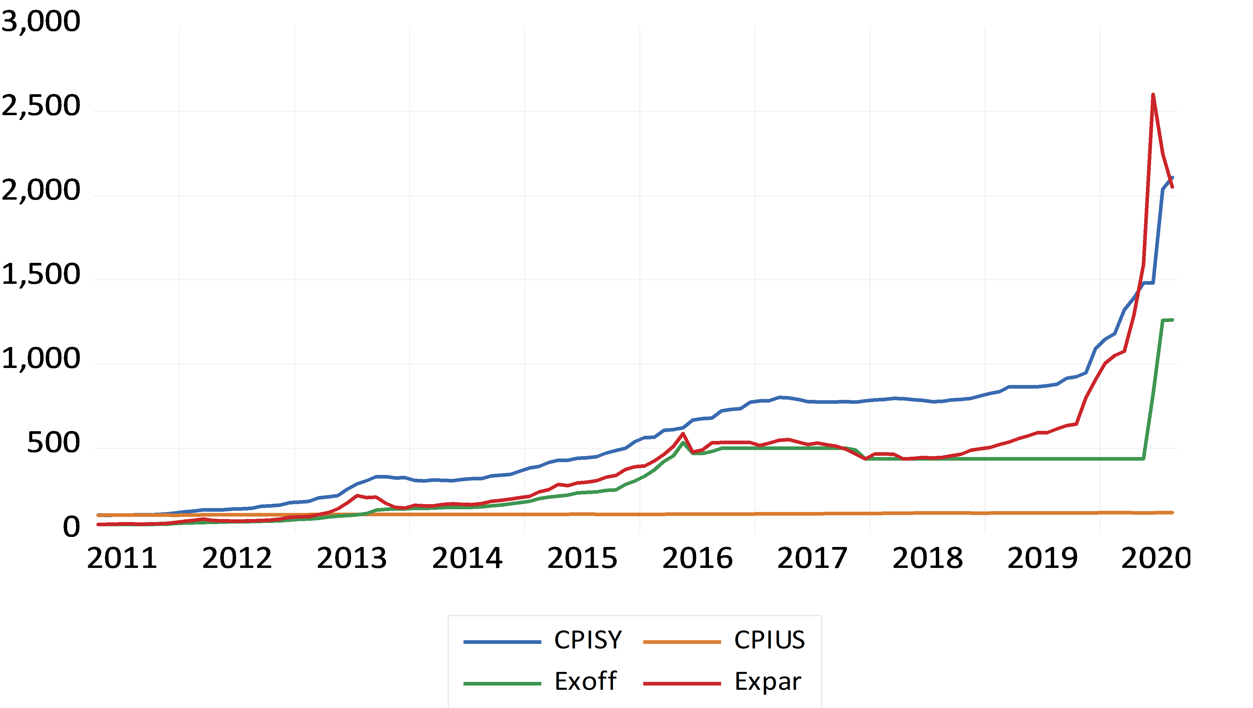
The current study makes three main contributions to the literature; first, it tests the validity of the PPP hypothesis by examining monthly real exchange rates of the Syrian pound against the US dollar over the period 2011:04-2020:08. This period is characterized by deterioration in the economic fundamentals and sharp currency depreciation as a result of the crisis that erupted on March 2011. Given developments in the official rate, the emergence of a parallel market, and a newly implemented intervention rate, the International Monetary Fund changed the classification of the exchange rate arrangement of Syria from “stabilized arrangement” to “other managed arrangement” on April 2011. Worth noting that Syria maintains during the period of study a multiple currency practice resulting from divergences of more than 2% between the official exchange rate and officially recognized market exchange rates [37].
Second, this study uses both the official and the parallel exchange rates in testing the PPP, which fills an important gap in the literature of PPP. In fact, studies concerning PPP mostly used the official exchange rates, especially in less developed countries. However, as outlined by Bahmani-Oskooee and Gelan, the official exchange rates may bias the inferences concerning the validity of PPP in the countries with significant black-market activities [21]. More specifically, due to restrictions on foreign currencies in Syria, these currencies are more expensive on the black market. The black-market or parallel exchange rate would thus reflect actual supply and demand pressures, and testing the validity of PPP in this context may indicate whether the foreign exchange market is efficient [38].
Third, in addition to conventional unit root tests, the nonlinear unit root tests of Kapetanios et al, Kruse, Kılıç and Sollis are applied to account for the possible nonlinearity that may arise from transaction costs, trade barriers and frequent official interventions in the foreign exchange market. As pointed out in Bahamani-Oskooee and Hegerty [38], nonlinear tests can be particularly useful in a study of less developed countries that face both external and internal shocks, such as periods of high inflation and sharp depreciation or devaluation of the exchange rate, which is the case of the Syrian economy. To our best knowledge, this study is the first that employs these nonlinear unit root tests to examine the validity of PPP for Syria over the period of crisis that erupted on March 2011.
The findings of this study should provide new evidence on the behavior of exchange rates in Syria during the recent period of crisis, which should be of interest to economists, policy makers and exchange rate market participants. As outlined by Taylor, the more important problem is to explain what drives the short-run dynamics of real exchange rates and how we account for the persistence of deviations from PPP in different time periods [39]. More specifically, knowing whether the PPP holds and if the real exchange rates follow a global stationary nonlinear process is important to specify the nature of chocks to the real exchange rate and the appropriate policy response.
MATERIALS AND METHODS
Data
To test the validity of PPP for Syria, the study applies monthly time series data of the natural logarithm of real exchange rate of the Syrian Pound against the US dollar from 2011:04 to 2020:08.
The importance of using the bilateral exchange rate against the dollar emerges from the fact that internal foreign exchange market is dollar dominated.
The real exchange rate is constructed as: RER =EX * (CPIUS / CPISY)
Where RER is the Real Exchange Rate, EX is the nominal Exchange Rate (measured as the price of the Syrian Pound relative to one unit of the US Dollar), and CPIUS and CPISY are the foreign and domestic consumer price indices (based on 2010=100), respectively.
We use both the official as well as the parallel real exchange rates against the US dollar. The real official exchange rate (RERoff) is constructed using the nominal official exchange rate (EXoff), while the real parallel exchange rate (RERPar) is constructed using the nominal parallel exchange rate (EXPar). All the series are plotted in Figure 1.
Data of the nominal exchange rates and the CPISY were collected from the Central Bank of Syria CBS (Data of the nominal official exchange rate were collected from the CBS website (available at https://www.cb.gov.sy/index.php?page=list&ex=2&dir=exchangerate&lang=1&service=4&act=1207). Data of the nominal parallel exchange rate (2011-0ctobre 2019) were obtained from the CBS upon request. Data of CPISY (2010=100) were collected from the CBS website for the period (2014:01-2020:08) (available at https://www.cb.gov.sy/index.php?page=list&ex= 2&dir=publications&lang=1&service=4&act=565). Data of CPISY (2010=100) for the period (2011:04-2013:12) were obtained from the CBS upon request because available data at the website are based on (2005=100) for this period. Note that data of CPISY are not available after 2020:08.). Data of the CPIUS were collected from the International Monetary Fund (Available at https://data.imf.org/regular.aspx?key=61015892).
Methods
To test the presence of a unit root in the exchange rate series, conventional unit root tests without structural breaks (ADF and PP) are first applied. However, these tests don’t take into account the presence of structural breaks in the data. In order to capture the structural breaks in the data, we employ the Lee and Strazicich one and two break unit root tests based on LM test.
While conventional and breakpoint unit root tests are applied, the data is assumed to be linear. Therefore, Kapetanios et al, Kruse, Kılıç and Sollis nonlinear unit root tests are applied based on the smooth transition autoregressive (STAR) model.
The Lee and Strazicich tests
Lee and Strazicich proposed using a minimum Lagrange Multiplier LM test for testing the presence of a unit root with one and two structural breaks. For this purpose, two models are considered; model A which allows for structural break in the intercept under the alternative hypothesis, and model C which allows for structural break in both the intercept and trend under the alternative hypothesis.
Nonlinear unit root test of Kapetanios et al
Kapetanios et al developed a procedure to detect the presence of non-stationarity against nonlinear but globally stationary exponential smooth transition autoregressive ESTAR processes. To this end, the following specific ESTAR model is used [16]:
∆yt= γyt-1[1-exp(-өy2t-1)] +ℇt (1)
Where ө (the slope parameter) is zero under the null hypothesis of unit root and positive under the alternative hypothesis of the stationary ESTAR process. Kapetanios et al. (2003) use first-order Taylor series approximation to the ESTAR model under the null and get the following auxiliary regression:
∆yt=δY3t-1+error (2)
Noting that the demeaned data is used for the case with nonzero mean, and the demeaned and detrended data for the case with nonzero mean and nonzero linear trend.
Assuming that the errors in equation 1 are serially correlated and that they enter in a linear fashion, then Kapetanios et al. (2003) extend model (1) to:
∆yt= j∆yt-j+ γyt-1[1-exp(-өy2t-1)] +ℇt (3)
The null hypothesis is tested against the alternative hypothesis by the tNL statistic:
tNL= /s.e ( ) (4)
Where δ ̂is the OLS estimate of δ and (s.e ( )) is the standard error of ( ) obtained from the following regression with p augmentation [16]:
∆yt= j∆yt-j+ δy3t-1+error (5)
With δ ̂is zero under the null hypothesis of unit root and negative under the alternative hypothesis.
Nonlinear unit root test of Kruse
Kruse extended the unit root test of Kapetanios et al by allowing for a nonzero attractor c in the exponential transition function. The degree of mean reversion of the real exchange rate depended on the distance of the lagged real exchange rate from this attractor [9].
To this end, he considers the following nonlinear time series model:
∆yt= γyt-1(1-exp {-ө (yt-1-c )2}) +ℇt (6)
As in Kapetanios et a, Kruse applied a first- order Taylor approximation around ө=0, and imposes β3 =0. The following regression was hence obtained:
∆yt= β1y3t-1+ β2y2t-1 +ut (7)
With ut being a noise term depending on ℇt.
In the regression 7, the null hypothesis of a unit root was H0: β1 = β2 = 0 and the alternative hypothesis of a globally stationary ESTAR process was H1: β1 < 0, β2 ≠ 0. Note that a standard Wald test wasn’t appropriate as one parameter is one-sided under H1 while the other one is two-sided [19]. To overcome this problem, Krus drived a modified Wald test that built up on the inference techniques by Abadir and Distaso [40]:
Ί=t2ß1/2=0+1( ˂0) t2ß1=0 (8)
Where t2ß1/2=0 represents the squared t-statistic for the hypothesis ß1/2= 0 with ß1/2 being orthogonal to β1. The second term t2ß1 is a squared t-statistic for the hypothesis β1 = 0.
Nonlinear unit root test of Kılıç
Kılıç considered an ESTAR model where the transition variable was the lagged changes of the dependent variable. Once appreciations or depreciations were large enough, real exchange rates may adjust towards equilibrium level due to profitable arbitrage.
The unit root test proposed was based on a one-sided t statistic where the t-statistic was optimized over the transition parameter space (γ). Kılıç specifies the following model, under the assumption that serially correlated errors entered in a linear way [24]:
∆yt= i∆yt-i+ Φyt-1[1-exp(-γz2t)] +ℇt (9)
With: Zt= ∆yt-d
The null and alternative hypotheses were set as H0: Φ= 0 against H1: Φ< 0.
As γ was unidentified under the unit root null hypothesis, Kılıç suggested to use the lowest possible t-value over a fixed parameter space of γ values that were normalized by the sample standard deviation of the transition variable zt.
Nonlinear unit root test of Sollis
ESTAR models assumed symmetrical adjustment in exchange rates towards PPP for the same size of a deviation, regardless of whether the real exchange rate was below or above the mean. However, appreciations and depreciations may lead to different speed of adjustment towards PPP [25].
Sollis proposed a test based on asymmetric exponential smooth transition autoregressive (AESTAR), where the speed of adjustment could be different below or above the threshold band.
The extended ESTAR process was as follows [25]:
∆yt=Φ1 y3t-1+Φ2 y4t-1+ i∆yt-i+ηi (10)
In the case of the rejection of the unit root hypothesis (Φ1= Φ2=0), the symmetric hypothesis, (Φ2=0) will be tested against the asymmetric alternative hypothesis, Φ2≠ 0. The hypothesis may be tested for the zero mean, non-zero mean and deterministic trend cases.
RESULTS
Prior to applying the nonlinear unit root tests, conventional linear unit root tests, which do not take into account any structural breaks, are first used. We initially employ the Augmented Dickey-Fuller (ADF) and the Phillips and Perron (PP). The null hypothesis is a unit root for these two tests.
The findings, presented in Table 1, indicate the random walk behavior of both the official and the parallel exchange rates series.
| Table 1: Conventional Linear Unit Root Tests Results | ||||
| ADF | PP | |||
| Constant | Constant and trend | Constant | Constant and trend | |
| LRERoff | -1.95 (0) | -2.28 (0) | -2.09 (2) | -2.29 (0) |
| LRERpar | -0.60 (3) | -1.96 (3) | -1.48 (7) | -3.03 (3) |
Source: Own computation (E-Views)
Notes: The lag length of the tests are reported in brackets. The optimal lag length of the ADF test was selected based on the modified AIC (MAIC). The bandwidth for the PP test were selected based on Newey-West automatic bandwidth selection procedure for a Bartlett kernel. The critical values for ADF and PP tests are -3.49 (1%), -2.89 (5%) and -2.58 (10%) for model with constant; and -4.05 (1%), -3.45 (5%) and -3.15 (10%) for the model with constant and trend.
To account for the power loss in the presence of structural breaks, we employ the Lee and Strazicich one and two break unit root tests. The relevance of using this approach is that it is unaffected by breaks under the null. According to the results reported in Table 2, we cannot reject the null hypothesis at the 5% level of significance, regardless of whether we use official or parallel official exchange rates. The null hypothesis could be rejected only for the official exchange rate after allowing for two breaks in the constant and trend and at the 10% level of significance. Note that the estimated break dates appear to vary concerning the model specification and data used.
These findings are consistent with those of Al-Ahmad and Ismaiel [36], who found that the unit root null hypothesis of Lumsdaine and Papell test could be rejected for the real effective exchange rates of the Syrian Pound only after allowing for three changes in the constant and trend and at the 10% level of significance.
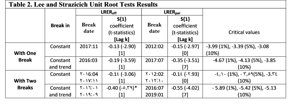 Source: Own computation (E-Views)
Notes: The coefficient of S{1} tests for the unit-root. The T-statistics are reported in brackets. The optimal lag length is determined by GTOS method. ***, **, * denote rejection of the null hypothesis of a unit root at 1%, 5% and 10% level of significance respectively.
We now test whether taking into account for non-linearity in the real exchange rates plays a role in analyzing unit root dynamics. Prior to this, we checked the nonlinearity of the series by using the conventional BDS test proposed by Broock et al [41]. According to the results, a nonlinear nature was detected in both series, which makes relevant to apply nonlinear unit root test (Results from the BDS test are not presented here but available upon request). To this end, we proceed with the non-linear unit root tests developed by Kapetanios et al. (2003), Kruse (2011), Kılıç (2011) and Sollis (2009). The results of test statistics are reported in Table 3.
| Table 3: Nonlinear Unit Root Tests Results | ||||||
| The nonlinear unit root test | LRERoff | LRERpar | Critical values | |||
| 1% | 5% | 10% | ||||
| Kapetanios et al. (2003) | Demeaned data | -5.82***(1) | -5.03***(1) | -3.48 | -2.93 | -2.66 |
| Detrended data | -6.58***(1) | -6.83***(1) | -3.93 | -3.40 | -3.13 | |
| Sollis (2009) | Demeaned data | 25.74***(1) | 16.51***(1) | 6.89 | 4.88 | 4.00 |
| Detrended data | 22.62 ***(1) | 23.18***(1) | 8.80 | 6.55 | 5.41 | |
| Kılıç (2011) | Demeaned data | -2.23*(1) | -1.58 (1) | -2.98 | -2.37 | -2.05 |
| Detrended data | -2.61**(1) | -2.99**(1) | -3.19 | -2.57 | -2.23 | |
| Kruse (2011) | Demeaned data | 44.35***(1) | 33.24***(1) | 13.75 | 10.17 | 8.60 |
| Detrended data | 42.97***(1) | 47.47***(1) | 17.10 | 12.82 | 11.10 | |
Source: Own computation (R for windows)
Notes: The lag length of the tests are reported in brackets. For all tests, the order of lags was chosen according to the Akaike information criterion (AIC). Table critical values of unit root tests are taken from KSS (2003)[16], Sollis (2009)[25], Kılıç (2011)[24] and Kruse (2011)[19]. ***, **, * denote rejection of the null hypothesis of a unit root at 1%, 5% and 10% level of significance respectively.
The results of Kapetanios et al and Kruse showed that the null of unit root was rejected at the 1% level of significance for both official and parallel exchange rate, regardless of whether we use model with demeaned or detrended data. We also rejected the null hypothesis for both series at the 1% level of significance of the (AESTAR) model of Sollis.
The test of Kılıç rejects the null hypothesis at the 5% level of significance for only the detrended data of both series. When demeaned data was used, the null of unit root test of Kılıç was rejected for only the official exchange rate and at the 10% level of significance. The test of
Kılıç hence provides stronger empirical support for nonlinear stationarity of the official exchange rate compared to parallel exchange rate. Non-linearity in the official exchange rates may rise, as suggested by Bahmani-Oskooee et al [42], from structural breaks due to official devaluation, besides frequent official interventions.
We note that Kılıç, which associates nonlinearity with the size of real exchange rate appreciation or depreciation, provided less evidence in favor of PPP compared to Kapetanios et al and Kruse, which allow for nonlinearity driven by the size of deviations from PPP. This finding contrasts with that of Yıldırım who found that the strongest evidence for PPP in Turkey is obtained through the unit root test of Kılıç [9].
DISCUSSION
Transaction costs and trade barriers are the plausible sources of nonlinearity in real exchange rates during the period of the study. It is important to note that the imposition of financial and economic sanctions has restricted exports and imports in Syria. (These sanctions include the freezing of Government of Syria assets, the cessation of transactions with individuals and companies in Syria, the termination of all investments supported by foreign Governments and the banning imports of Syrian oil). Indeed, the great government spending on nontraded goods compared to traded goods during the period of crisis has increased the share of nontraded goods.
The nonlinearity of exchange rate series may also arise from frequent official interventions in the foreign exchange market. In fact, the continuous deterioration in the economic fundamentals, in addition to the speculative pressure and the capital flight have contributed to sharp depreciation of the Syrian pound during the period of crisis, which authority tried to counter through increasing the interventions. These interventions could lead to non-linearity into the adjustment of the nominal exchange rate and, with price stickiness in the short run, the adjustment of the real exchange rate as well [1,42]. Note that, as stated in Dutta and Leon [43], policymakers in less developed countries prefer having longer periods of currency appreciation than depreciation, even though the economic fundamentals would require the opposite. This could be explained by fear of inflation (pass-through from exchange rate swings to inflation) and currency mismatches.
The high level of inflation could be another possible contributor to adjustment of real exchange rates series. The annual inflation rate in Syria reached 163.1% in December 2020 compared to the base year 2010, the year before the eruption of the Syrian crisis [44]. This implies, as argued by Cashin and Mcdermott [34], more frequent adjustment of goods prices, which could reduce the duration of deviation from PPP. Note that as prices have less of a tendency to move downwards, the exchange rate might have to do more of the adjusting. An adjustment might thus be asymmetric between the upward and downward deviations from equilibrium [38].
Our results can also provide some evidence on how the monetary authority in Syria reacted in the period of crisis. According to IFM reports, the exchange rate classification of Syria was changed from “stabilized arrangement” to “other managed management” on April 2011, in the aftermath of the crisis that erupted on March 2011 [37]. This means moving to more flexible exchange rate regime. In 2012, the prime minister issued the law No. 1131 which stated the movement towards a free exchange rate regime, with the right of the Central Bank of Syria to intervene in the exchange market to correct the exchange rate trends in the market. We believe that moving to a more market-oriented exchange rate has facilitated the nominal exchange rate adjustment. As discussed in Cashin and Mcdermott [34], more flexibility in nominal exchange rates may increase the speed of the parity reversion of real exchange rates by encouraging more frequent adjustment of goods prices. These findings are consistent with those of Baharumshah et al, as they found that the weak form of PPP holds for six East-Asian countries only over the post-crisis period [45]. They suggest that the evidence in favor of PPP was stronger following the financial crisis when countries had to abandon pegging their exchange rates. We also believe that interventions in the foreign exchange market have some justification as the deviations of real exchange rates from the equilibrium appear to be temporary and the exchange rates are adjustable towards PPP.
CONCLUSION AND RECOMMENDATION
This study investigates the PPP hypothesis for Syria over the period (2011:04-2020:08), using both official and parallel real exchange rates of the Syrian Pound against the US Dollar. To this end, a battery of nonlinear unit root tests is adopted along with popular conventional unit root tests.
The conventional tests (ADF and PP) fail to reject the null of a unit root for the real exchange rate series at the 5% level of significance, regardless of whether we use official or parallel exchange rate. The non-stationarity of both series is robust to the existence of breaks since the Lee and Strazicich unit root tests fail to reject the null hypothesis at the 5% level of significance for both official and parallel series.
When nonlinearity is incorporated in the testing procedure, the nonlinear tests of Kapetanios et al, Kruse, and Sollis support PPP for both real exchange rate series under consideration at the 1% level of significance. The test of Kılıç supports PPP only after allowing for a trend in both series and at the 5% level of significance.
The findings of this study provide new evidence on the behavior of exchange rates in Syria during the recent period of crisis. The non-linear mean reversion indicates that as the real exchange rate deviates from its long-run equilibrium, it tends to have faster speed of adjustment. This implies that PPP can be used to determine whether the currency is overvalued or undervalued, and investors and speculators are not able to obtain unbounded gains from arbitrage [9,45].
Finally, as our results signify the importance of non-linear adjustment in real exchange rates, it is so important that policymakers and exchange rate market participants take account of possibility of nonlinear dynamics in their decisions. Future research should also take on the issue of nonlinearity of real exchange rate more seriously when examining the PPP.
Nowcasting GDP in Parsimony Data Environment Using Bayesian Mixed Frequency VAR (Empirical Evidence from Syria)
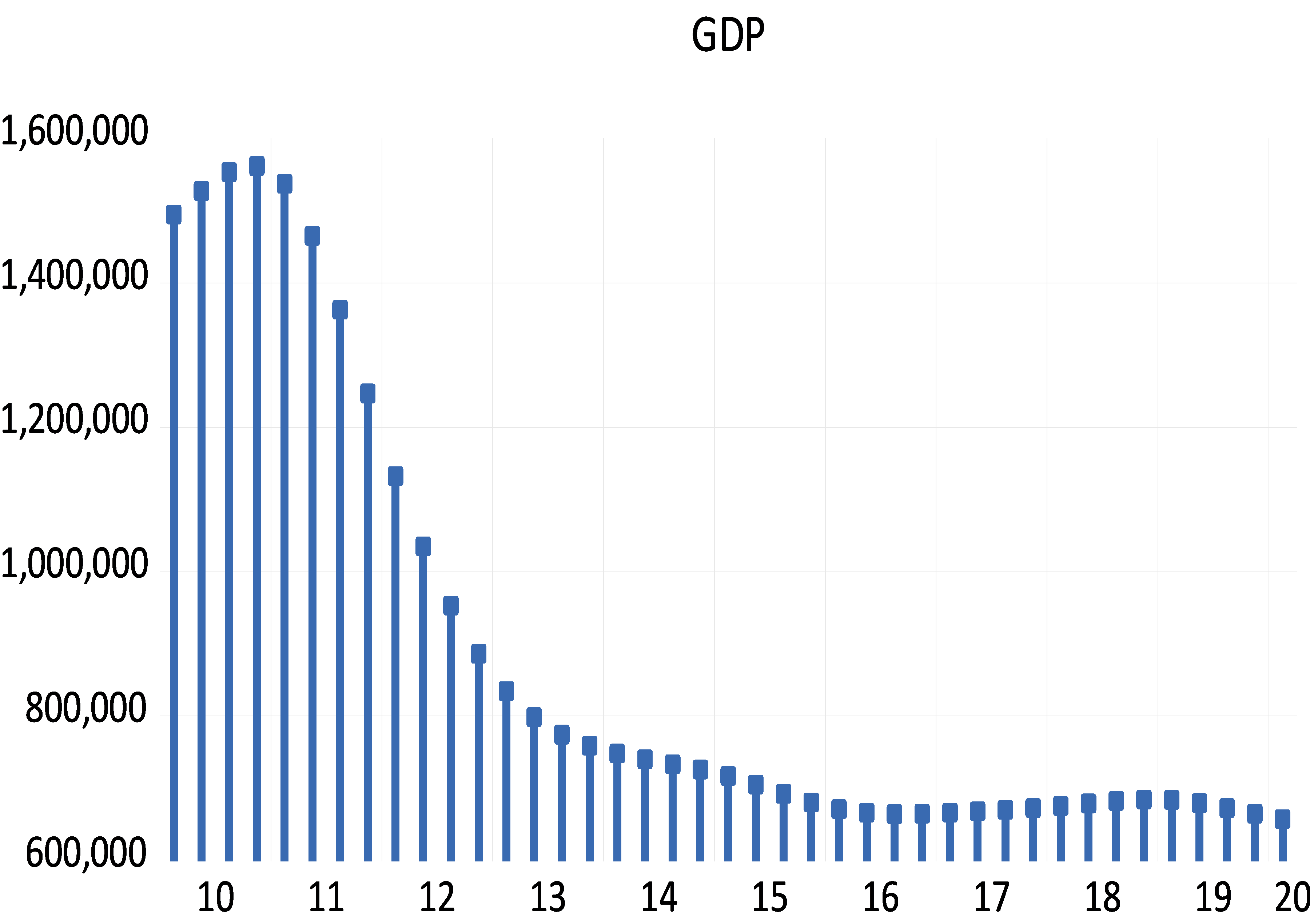
INTRODUCTION
Nowcasting refers to the projection of information about the present, the near future, and even the recent past. The importance of nowcasting has shifted from weather forecasting to economics, where economists use it to track the economy status through real-time GDP forecasts, as it is the main low-frequency (quarterly – annually) indicator reflecting the state of the country’s economy. This is like satellites that reflect the weather on earth. It does this by relying on high-frequency measured variables (daily – monthly) that are reported in real-time. The importance of using nowcasting in the economy stems from the fact that data issuers, statistical offices and central banks release the main variables of the economy, such as gross domestic product and its components, with a long lag. In some countries, it may take up to five months. In other countries, it may take two years depending on the capabilities each country has, leading to a state of uncertainty about the economic situation among economic policy makers and state followers business. Real-time indicators related to the economy (e.g consumer prices and exchange rates) are used here in order to obtain timely information about variables published with a delay. The first use of nowcasting technology in economics dates back to Giannone et al 2008, by developing a formal forecasting model that addresses some of the key issues that arise when using a large number of data series released at varying times and with varying delays [1]. They combine the idea of “bridging” the monthly information with the nowcast of quarterly GDP and the idea of using a large number of data releases in a single statistical framework. Banbura et al proposed a statistical model that produces a series of Nowcasting forecasts on real-time releases of various economic data [2]. The methodology enables the processing of a large amount of information from nowcasting’s Eurozone GDP Q4 2008 study. Since that time, the models that can be used to create nowcasting have expanded. Kuzin et al compared the mixed-frequency data sampling (MIDAS) approach proposed by Ghysels et al [4,5] with the mixed-frequency VAR (MF-VAR) proposed by Zadrozny and Mittnik et al [6,7], with model specification in the presence of mixed-frequency data in a policy-making situation, i.e. nowcasting and forecasting quarterly GDP growth in Eurozone on a monthly basis. After that time, many econometric models were developed to allow the use of nowcasting and solve many data problems. Ferrara et al [8] proposed an innovative approach using nonparametric methods, based on nearest neighbor’s approaches and on radial basis function, to forecast the monthly variables involved in the parametric modeling of GDP using bridge equations. Schumacher et al [9] compare two approaches from nowcasting GDP: Mixed Data Sampling (MIDAS) regressions and bridge equations. Macroeconomics relies on increasingly non-standard data extracted using machine learning (text analysis) methods, with the analysis covering hundreds of time series. Some studies examined US GDP growth forecasts using standard high-frequency time series and non-standard data generated by text analysis of financial press articles and proposed a systematic approach to high-dimensional time regression problems [10-11]. Another team of researchers worked on dynamic factor analysis models for nowcasting GDP [12], using a Dynamic Factor Model (DFM) to forecast Canadian GDP in real-time. The model was estimated using a mix of soft and hard indices and the authors showed that the dynamic factor model outperformed univariate criteria as well as other commonly used nowcasting models such as MIDAS and bridge regressions. Anesti et al [13] proposed a release-enhanced dynamic factor model (RA-DFM) that allowed quantifying the role of a country’s data flow in the nowcasting of both early (GDP) releases and later revisions of official estimates. A new mixed-frequency dynamic factor model with time-varying parameters and random fluctuations was also designed for macroeconomic nowcasting, and a fast estimation algorithm was developed [14]. Deep learning models also entered the field of GDP nowcasting, as in many previous reports [15-17]. In Syria, there are very few attempts to nowcasting GDP, among which we mention a recent report that uses the MIDAS Almon Polynomial Weighting model to nowcasting Syria’s annual GDP based on the monthly inflation rate data [18]. Our research aims to solve a problem that exists in the Arab and developing countries in general, and Syria in particular, namely the inability to collect data in real-time on the main variable in the economy due to the weakness of material and technical skills. Therefore, this study uses Bayesian mixed-frequency VAR models to nowcast GDP in Syria based on a set of high-frequency data. The rationale for choosing these models is that they enable the research goal to be achieved within a structural economic framework that reduces statistical uncertainty in the domain of high-dimensional data in a way that distinguishes them from the nowcasting family of models, according to a work by Cimadomo et al and Crump et al [19-20]. The first section of this research includes the introduction and an overview of the previous literature. The second section contains the research econometric framework, through which the architecture of the research model is developed within a mathematical framework. The third section is represented by the data used in the research including the exploratory phase. The fourth section contains the discussion and interpretation of the results of the model after the evaluation. The fifth section presents the results of the research and proposals that can consider a realistic application by the authorities concerned.
MATERIALS AND METHODS
The working methodology in this research is divided into two main parts. The first in which the low-frequency variable (Gross Domestic Product) is converted from annual to quarterly with the aim of reducing the forecast gap and tracking the changes in the GDP in Syria in more real-time., by reducing the gap with high-frequency data that we want to predict their usage. To achieve this, we used Chow-Lin’s Litterman: random walk variant method.
Chow-Lin’s Litterman Method
This method is a mix and optimization of two methods. The Chow-Lin method is a regression-based interpolation technique that finds values of a series by relating one or more higher-frequency indicator series to a lower-frequency benchmark series via the equation:
x(t)=βZ(t)+a(t) (1)
Where is a vector of coefficients and a random variable with mean zero and covariance matrix Chow and Lin [21] used generalized least squares to estimate the covariance matrix, assuming that the errors follow an AR (1) process, from a state space model solver with the following time series model:
a(t)=ρa(t-1)+ϵ(t) (2)
Where ϵ(t)~N(0,σ^2) and |ρ|<1. The parameters ρ and βare estimated using maximum likelihood and Kalman filters, and the interpolated series is then calculated using Kalman smoothing. In the Chow-Lin method, the calculation of the interpolated series requires knowledge of the covariance matrix, which is usually not known. Different techniques use different assumptions about the structure beyond the simplest (and most unrealistic) case of homoscedastic uncorrelated residuals. A common variant of Chow Lin is Litterman interpolation [22], in which the covariance matrix is computed from the following residuals:
a(t)=a(t-1)+ϵ(t) (3)
Where ϵ(t)~N(0,V)
ϵ(t)=ρϵ(t-1)+e(t) (4)
and the initial state a(0)=0. . This is essentially an ARIMA (1,1,0) model.
In the second part, an econometric model suitable for this study is constructed by imposing constraints on the theoretical VAR model to address a number of statistical issues related to the model’s estimation, represented by the curse of dimensions.
Curse of Dimensions
The dimensional curse basically means that the error increases with the number of features (variables). A higher number of dimensions theoretically allows more information to be stored, but rarely helps as there is greater potential for noise and redundancy in real data. Collecting a large number of data can lead to a dimensioning problem where very noisy dimensions can be obtained with less information and without much benefit due to the large data [23]. The explosive nature of spatial scale is at the forefront of the Curse of Dimensions cause. The difficulty of analyzing high-dimensional data arises from the combination of two effects: 1- Data analysis tools are often designed with known properties and examples in low-dimensional spaces in mind, and data analysis tools are usually best represented in two- or three-dimensional spaces. The difficulty is that these tools are also used when the data is larger and more complex, and therefore there is a possibility of losing the intuition of the tool’s behavior and thus making wrong conclusions. 2- The curse of dimensionality occurs when complexity increases rapidly and is caused by the increasing number of possible combinations of inputs. That is, the number of unknowns (parameters) is higher than the number of observations. Assuming that m denotes dimension, the corresponding covariance matrix has m (m+1)/2 degrees of freedom, which is a quadratic term in m that leads to a high dimensionality problem. Accordingly, by imposing a skeletal structure through the initial information of the Bayesian analysis, we aimed to reduce the dimensions and transform the high-dimensional variables into variables with lower dimensions and without changing the specific information of the variables. With this, the dimensions were reduced in order to reduce the feature space considering a number of key features.
Over Parameterizations
This problem, which is an integral part of a high dimensionality problem, is statistically defined as adding redundant parameters and the effect is an estimate of a single, irreversible singular matrix [24]. This problem is critical for statistical estimation and calibration methods that require matrix inversion. When the model starts fitting the noise to the data and the estimation parameters, i.e. H. a high degree of correlation existed in the co-correlation matrix of the residuals, thus producing predictions with large out-of-sample errors. In other words, the uncertainty in the estimates of the parameters and errors increases and becomes uninterpretable or far from removed from the realistic estimate. This problem is addressed by imposing a skeletal structure on the model, thereby transforming it into a thrift. Hence, it imposes constraints that allow a correct economic interpretation of the variables, reducing the number of unknown parameters of the structural model, and causing a modification of the co – correlation matrix of the residuals so that they become uncorrelated with some of them, in other words, become a diagonal matrix.
Overfitting and Underfitting
Overfitting and Underfitting are major contributors to poor performance in models. When Overfitting the model (which works perfectly on the training set while ineffectively fitting on the test set), it begins with matching the noise to the estimation data and parameters, producing predictions with large out-of-sample errors that adversely affect the model’s ability to generalize. An overfit model shows low bias and high variance [25]. Underfitting refers to the model’s inability to capture all data features and characteristics, resulting in poor performance on the training data and the inability to generalize the model results [26]. To avoid and detect overfitting and underfitting, we tested the validity of the data by training the model on 80% of the data subset and testing the other 20% on the set of performance indicators.
Theoretical VAR model
VAR model developed by Sims [27] has become an essential element in empirical macroeconomic research. Autoregressive models are used as tools to study economic shocks because they are based on the concept of dynamic behavior between different lag values for all variables in the model, and these models are considered to be generalizations of autoregressive (AR) models. The p-rank VAR is called the VARp model and can be expressed as:
y_t=C+β_1 y_(t-1)+⋯+β_P y_(t-P)+ϵ_t ϵ_t~(0,Σ) (5)
Where y_t is a K×1 vector of endogenous variables. Is a matrix of coefficients corresponding to a finite lag in, y_t, ϵ_t: random error term with mean 0 representing external shocks, Σ: matrix (variance–covariance). The number of parameters to be estimated is K+K^2 p, which increases quadratic with the number of variables to be included and linearly in order of lag. These dense parameters often lead to inaccuracies regarding out-of-sample prediction, and structural inference, especially for high-dimensional models.
Bayesian Inference for VAR model
The Bayesian approach to estimate VAR model addresses these issues by imposing additional structure on the model, the associated prior information, enabling Bayesian inference to solve these issues [28-29], and enabling the estimation of large models [2]. It moves the model parameters towards the parsimony criterion and improves the out-of-sample prediction accuracy [30]. This type of contraction is associated with frequentist regularization approaches [31]. Bayesian analysis allows us to understand a wide range of economic problems by adding prior information in a normal way, with layers of uncertainty that can be explained through hierarchical modelling [32].
Prior Information
The basic premise for starting a Bayesian analysis process must have prior information, and identifying it correctly is very important. Studies that try not to impose prior information result in unacceptable estimates and weak conclusions. Economic theory is a detailed source of prior information, but it lacks many settings, especially in high-dimensional models. For this reason, Villani [33] reformulates the model and places the information at a steady state, which is often the focus of economic theory and which economists better understand. It has been proposed to determine the initial parameters of the model in a data-driven manner, by treating them as additional parameters to be estimated. According to the hierarchical approach, the prior parameters are assigned to hyperpriors. This can be expressed by the following Bayes law: 
Wherey= (y_(p+1)+⋯+y_T)^T,θ: is coefficients AR and variance for VAR model, γ: is hyperparameters. Due to the coupling of the two equations above, the ML of the model can be efficiently calculated as a function of γ. Giannone et al [34] introduced three primary information designs, called the Minnesota Litterman Prior, which serves as the basis, the sum of coefficients [35] and single unit root prior [36].
Minnesota Litterman Prior
Working on Bayesian VAR priors was conducted by researchers at the University of Minnesota and the Federal Reserve Bank of Minneapolis [37] and these early priors are often referred to as Litterman prior or Minnesota Prior. This family of priors is based on assumption that Σ is known; replacing Σwith an estimate Σ. This assumption leads to simplifications in the prior survey and calculation of the posterior.
The prior information basically assumes that the economic variables all follow the random walk process. These specifications lead to good performance in forecasting the economic time series. Often used as a measure of accuracy, it follows the following torques:

The key parameter ⋋ is which controls the magnitude influence of the prior distribution, i.e. it weighs the relative importance of the primary data. When the prior distribution is completely superimposed, and in the case of the estimate of the posterior distributions will approximate the OLS estimates. is used to control the break attenuation, and is used to control the prior standard deviation when lags are used. Prior Minnesota distributions are implemented with the goal of de-emphasizing the deterministic component implied by the estimated VAR models in order to fit them to previous observations. It is a random analysis-based methodology for evaluating systems under non-deterministic (stochastic) scenarios when the analytical solutions are complex, since this method is based on sampling independent variables by generating phantom random numbers.
Dummy Observations
Starting from the idea of Sims and Zha [38] to complement the prior by adding dummy observations to the data matrices to improve the predictive power of Bayesian VAR. These dummy observations consist of two components; the sum-of-coefficient component and the dummy-initial-observation component. The sum-of-coefficients component of a prior was introduced by Doan et al [37] and demonstrates the belief that the average of lagged values of a variable can serve as a good predictor of that variable. It also expresses that knowing the average of lagged values of a second variable does not improve the prediction of the first variable. The prior is constructed by adding additional observations to the top (pre-sample) of the data matrices. Specifically, the following observations are constructed: 
Where is the vector of the means over the first observed by each variable, the key parameter is used to control for variance and hence the impact of prior information. When the prior information becomes uninformative and when the model is formed into a formula consisting of a large number of unit roots as variables and without co-integration. The dummy initial observation component [36] creates a single dummy observation that corresponds to the scaled average of the initial conditions, reflecting the belief that the average of the initial values of a variable is likely to be a good prediction for that variable. The observation is formed as:

Where is the vector of the means over the first observed by each variable, the key parameter is used to control on variance and hence the impact of prior information. As , all endogenous variables in VAR are set to their unconditional mean, the VAR exhibits unit roots without drift, and the observation agrees with co-integration.
Structural Analysis
The nowcasting technique within the VAR model differs from all nowcasting models in the possibility of an economic interpretation of the effect of high-frequency variables on the low-frequency variable by measuring the reflection of nonlinear changes in it, which are defined as (impulse and response). A shock to the variable not only affects the variable directly, but it is also transmitted to all other endogenous variables through the dynamic (lag) structure of VAR. An impulse response function tracks the impact of a one-off shock to one of the innovations on current and future values of the endogenous variable.
BVAR is estimated reductively, i.e., without a contemporary relationship between endogenous variables in the system. While the model summarizes the data, we cannot determine how the variables affect each other because the reduced residuals are not orthogonal. Recovering the structural parameters and determining the precise propagation of the shocks requires constraints that allow a correct economic interpretation of the model, identification constraints that reduce the number of unknown parameters of the structural model, and lead to a modification of the co-correlation matrix of the residuals so that they become uncorrelated, i.e., they become a diagonal matrix. This problem is solved by recursive identification and achieved by Cholesky’s analysis [39] of the variance and covariance matrix of the residuals , Where Cholesky uses the inverse of the Cholesky factor of the residual covariance matrix to orthogonalize the impulses. This option enforces an ordering of the variables in the VAR and attributes the entire effect of any common component to the variable that comes first in the VAR system. For Bayesian frame, Bayesian sampling will use a Gibbs or Metropolis-Hasting sampling algorithm to generate draws from the posterior distributions for the impulse. The solution to this problem can be explained mathematically from the VAR model:
![]()
Where show us contemporaneous correlation. Coefficient matrix at lag1, error term where:

In order to estimate the previous equation, we must abandon the contemporaneous relations between the endogenous variables since we transfer them to the other side:

Now parsimony VAR model can be estimated:
![]()
Where A_1 are reduced coefficient. u_t Represent the weighted averages of the structural coefficientsβ_1,ϵ_t. Where:
 Mixed Frequency VAR
Complementing the constraints imposed on the theoretical VAR model, as a prelude to achieving the appropriate form for the research model and developing the model presented by AL-Akkari and Ali [40] to predict macroeconomic data in Syria, we formulate the appropriate mathematical framework for the possibility to benefit from high-frequency data emitted in real-time in nowcasting of GDP in Syria.
We estimate a mixed frequency VAR model with no constant or exogenous variables with only two data frequencies, low and high (quarterly-monthly), and that there are high frequency periods per low frequency period. Our model consists of variable observed at low frequency and variables observed at high frequency. Where:
: represent the low-frequency variable observed during the low-frequency period .
: represent the high-frequency variable observed during the low-frequency period .
By stacking the and variables into the matrices and ignoring the intersections and exogenous variables for brevity, respectively, we can write the VAR:

Performance indicators
We use indicators to assess the performance of the models which are used to determine their ability to explain the characteristics and information contained in the data. It does this by examining how closely the values estimated from the model correspond to the actual values, taking into account the avoidance of an underfitting problem that may arise from the training data and an overfitting problem that arises from the test data. The following performance indicators include:
Theil coefficient (U):
 Mean Absolute Error (MAE):
![]()
Root Mean Square Error (RMSE): 
Where the forecast is value; is the actual value; and is the number of fitted observed. The smaller the values of these indicators, the better the performance of the model.
RESULTS & DISCUSSION
As mentioned, the data consists of high and low frequency variables collected from the websites of official Syrian organizations and the World Bank [41-46], summarized in Table 1, which shows basic information about data. The data of the variable GDP were collected annually and converted using the combination of Chow-Lin’s Litterman methods, (Fig 1), which shows that the volatility in annual GDP was explained by the quarter according to the hybrid method used, and gives us high reliability for the possibility of using this indicator in the model. For high-frequency data, the monthly closing price was collected from the sources listed in Table (1) and its most recent version was included in the model to provide real-time forecasts.

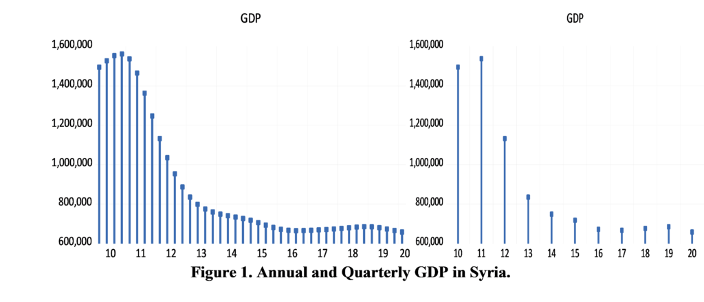
Figure (2) shows the evolution of these variables. We presented in Figure (2), the data in its raw form has a general stochastic trend and differs in its units of measurement. To unify the characteristics of this data, growth rates were used instead of prices in this case, or called log, because of their statistical properties. These features are called stylized facts; first, there is no normal distribution. In most cases, the distribution deviates to the left and has a high kurtosis. It has a high peak and heavy tails [47]. Second, it has the property of stationary and there is almost no correlation between the different observations [48]. The log of this series is calculated.
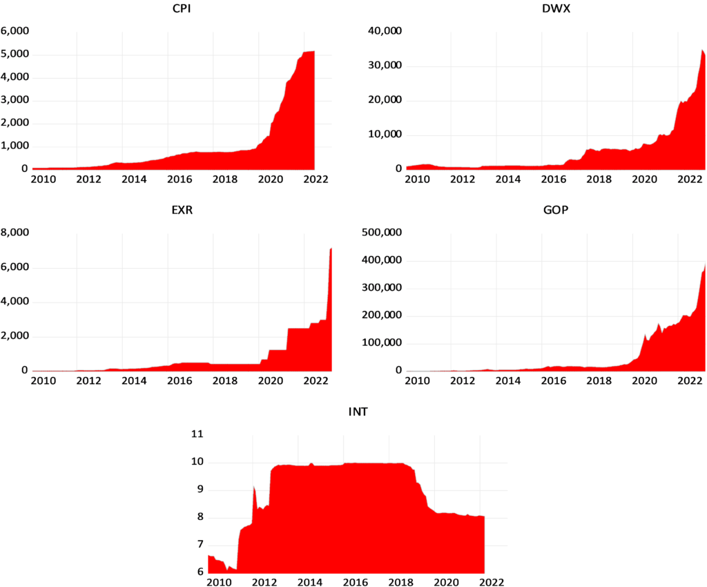
Figure 2. Evolution of high frequency study variables
Figure (3) shows the magnitude growth of the macroeconomic and financial variables in Syria during the indicated period. We note that the data is characterized by the lack of a general trend and volatility around a constant. We found that the fluctuations change over time and follow the characteristic of stochastic volatility that decreases, increases and then decreases. We found that the most volatile variable is the exchange rate (EXR) and the period between 2019 and 2020 is the one when the variables fluctuated the most due to uncertainty and US economic sanctions. We also noted that the periods of high volatility are offset by negative growth in Syria’s GDP. Using the following Table (2), we show the most important descriptive statistics for the study variables.
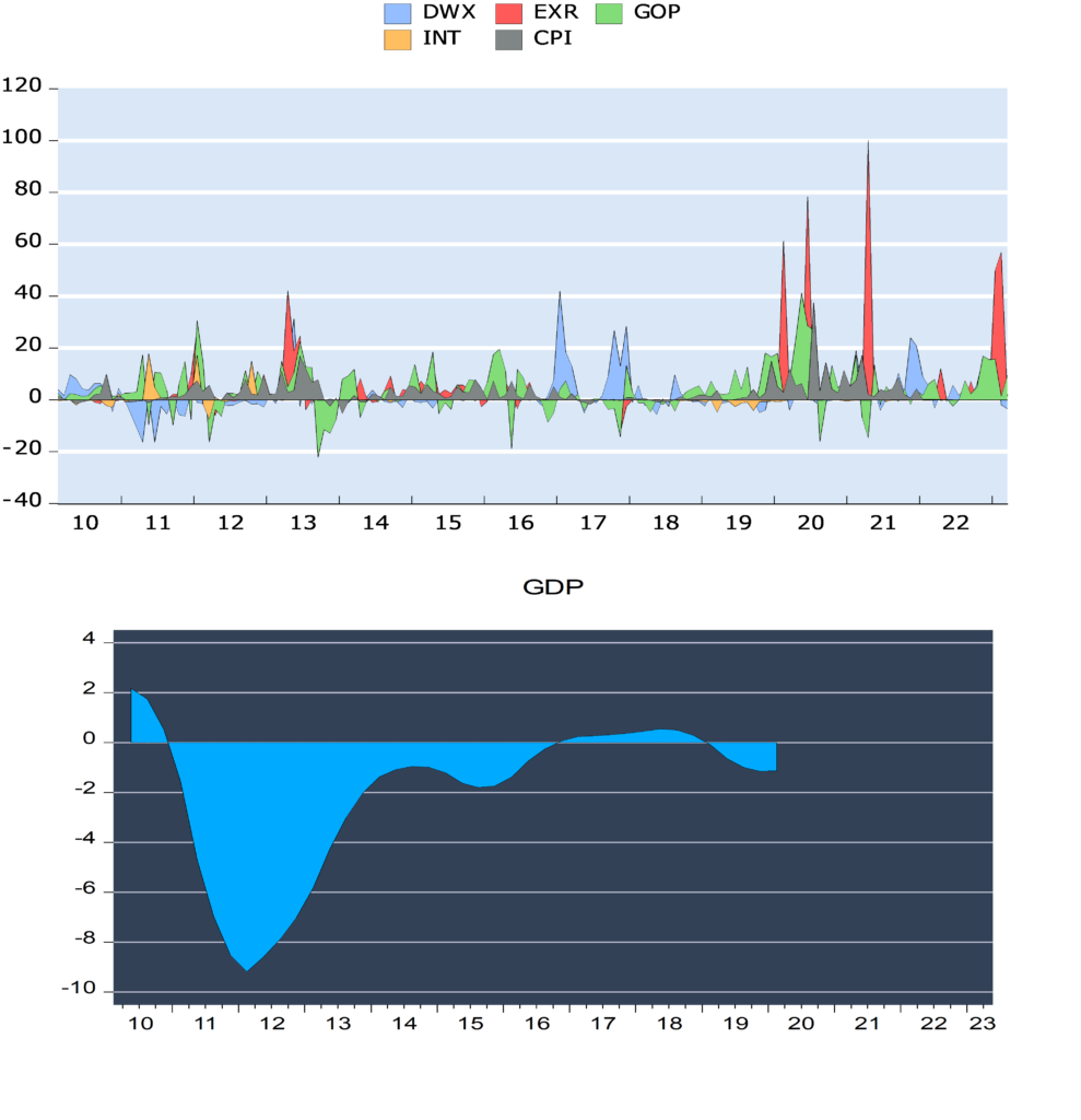

*** denotes the significance of the statistical value at 1%. ** at 5%. * at 10%.
Table (2) shows that the probability value of the normal distribution test statistic is significant at 1%, and we conclude that the data on the growth rates of the Syrian economy is not distributed according to the normal distribution, and both the mean and the standard deviation were not useful for the prediction in this case since they have become a breakdown. We also note from Table (2) the positive value of the skewness coefficient for all variables, and therefore the growth rates of economic variables are affected by shocks in a way that leads to an increase in the same direction, except for the economic growth rate, in which the shocks are negative and the distribution is skewed to the left. We also found that the value of the kurtosis coefficient is high (greater than 3 for all variables), indicating a tapered leptokurtic-type peak. Additionally, we noted that the largest difference between the maximum and minimum value of the variable is the exchange rate, which indicates the high volatility due to the devaluation of the currency with the high state of uncertainty after the start of the war in Syria. Also, one of the key characteristics of growth rates is that they are stable (i.e. they do not contain a unit root). Since structural changes affect expectations, as we have seen in Figure (1), there is a shift in the path of the variable due to political and economic events. We hence used the breakpoint unit root test proposed by Perron et al [49-50], where we assume that the structural change follows the course of innovation events and we test the largest structural breakpoint for each variable and get the following results:
![]()
Where is break structural coefficients, is dummy variable indicated on structural change, : intercept, : lag degree for AR model. Figure (4) shows the structural break estimate for the study variables. Structural break refers to a change in the behavior of a variable over time, shifting relationships between variables. Figure (4) also demonstrates that all macroeconomic variables have suffered from a structural break, but in different forms and at different times, although they show the impact of the same event, namely the war in Syria and the resulting economic blockade by Arab and Western countries, as all structural breaks that have occurred after 2011. We found that in terms of the rate of economic growth, it has been quickly influenced by many components and patterns. For EXR, CPI, GOP, the point of structural change came after 2019, the imposition of the Caesar Act and the Corona Pandemic in early 2020, which resulted in significant increases in these variables. We noted that the structural break in the Damascus Stock Exchange Index has occurred in late 2016 as the security situation in Syria improved, resulting in restored investor confidence and realizing returns and gains for the market.
The step involves imposing the initial information on the structure of the model according to the properties of the data. Based on the results of the exploratory analysis, the prior Minnesota distributions were considered a baseline, and the main parameter is included in the hierarchical modeling:
Rho H = 0.2 is high frequency AR(1), Rho L = 0 is low frequency AR(1), Lambda = 5 is overall tightness, Upsilon HL = 0.5 is high-low frequency scale, Upsilon LH = 0.5 is low-high frequency scale, Kappa = 1 is exogenous tightness. C1 = 1 is residual covariance scale. The number of observations in the frequency conversion specifies the number of high frequency observations to use for each low frequency period. When dealing with monthly and quarterly data, we can specify that only two months from each quarter should be used. Last observations indicate that the last set of high-frequency observations from each low-frequency period should be used. Initial covariance gives the initial estimate of the residual covariance matrix used to formulate the prior covariance matrix from an identity matrix, specifying the number of Gibbs sampler draws, the percentage of draws to discard as burn-in, and the random number seed. The sample is divided into 90% training (in–of –sample) and 10% testing data (out-of–sample).
![]()
Table (3) provides us with the results of estimating the model to predict quarterly GDP in Syria. The results show the basic information to estimate the prior and posterior parameters, and the last section shows the statistics of the models such as the coefficient of determination and the F-statistic. We note that every two months were determined from a monthly variable to forecast each quarter of GDP in the BMFVAR model. Although there is no explanation due to the imposition of constraints, the model shows good prediction results with a standard error of less than 1 for each parameter and a high coefficient of determination of the GDP prediction equation explaining 93.6% of the variance in GDP.

Figure (5) also shows us the reliability of the prediction results. It is clear that the roots of the estimation of the parameters follow the inverse AR polynomial process. The inverted AR roots have modules very close to one which is typical of many macro time series models.
Table (4) shows the evolution of GDP Forecasting in Syria in and out the sample based on a number of indicators. When the value of these indicators is close to 0, the estimated values are close to the actual values, which is shown by Table 4, since the values of these indicators are all less than 1. The out-of-sample predicted values show a better performance of the model, and hence it can be adopted to track changes in quarterly GDP over time. Up-to-date with current versions.
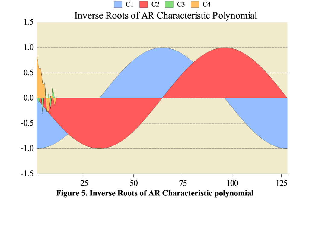
Through the data visualization technique, Figure (6) shows us the closeness of the expected values of quarterly GDP in Syria in of sample, which leads to the exclusion of the presence of an undue problem in the estimate (overfitting – underfitting). The median is used in the prediction because it is immune to the values of structural breaks and the data are not distributed according to the normal distribution. The out-of-sample forecast results (Fig 7) also indicate negative rates of quarterly GDP growth in Syria with the negative impact of internal and external shocks on the Syrian economy with the accumulation of the impact of sanctions, the lack of long-term production plans and the ineffectiveness of internal monetary policy tools, as the latest forecasts for GDP growth this quarter are (-3.69%).
The uncertainty at each point in time is included in the Syrian GDP projections, thereby achieving two objectives: incorporating the range of GDP change at each point in time and knowing the amount of error in the forecasts. We found that uncertainty increases as the forecast period lengthens (Figures 8-10).
The model also provides us with important results through scenario analysis. Figure 11 shows that the quarterly GDP in Syria is affected by the shocks of high-frequency variables, since this Figure shows that the shocks have negative impacts. This recommends a better activation of the instruments of The Central Bank and those responsible for monetary policy in Syria. These results are considered important tools for them to know and evaluate the effectiveness of their tools.
Figure 6. Forecasting quarterly GDP in Syria in of sample with 35%, 10%, 5% distribution quantities.
Figure 7. Forecasting quarterly GDP in Syria out of sample with 35%, 10%, 5% distribution quantities.

Figure 8. Uncertainty for forecasting quarterly GDP in Syria in-of –sample
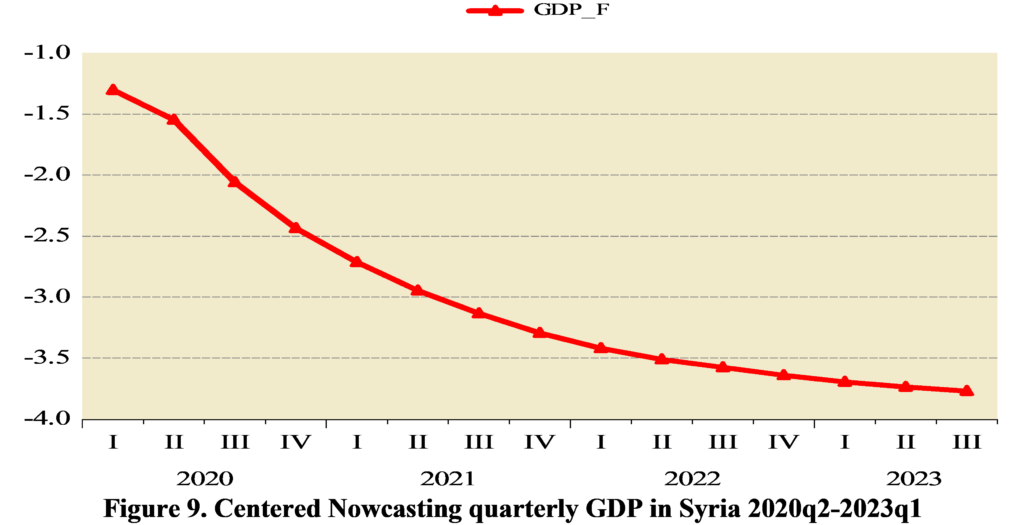

Figure 10. Uncertainty for forecasting quarterly GDP in Syria out-of –sample
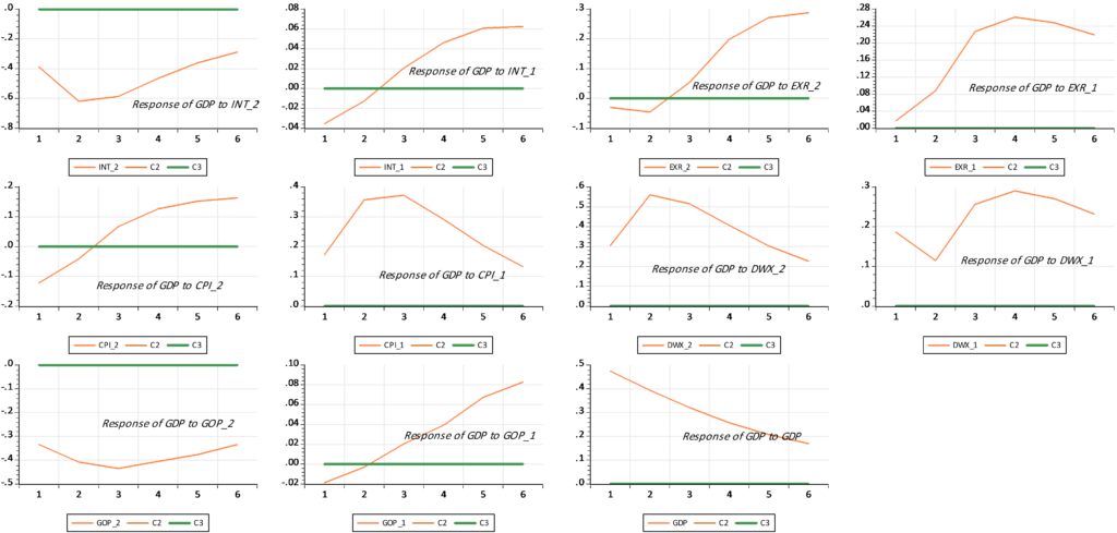
Figure 11. Shocks of high-frequency variables in the quarterly GDP of Syria
CONCLUSIONS AND RECOMMENDATIONS
This paper showed that BMFVAR could be successfully used to handle Parsimony Environment Data, i.e., a small set of macroeconomic time series with different frequencies, staggered release dates, and various other irregularities – for real-time nowcasting. BMFVAR are more tractable and have several other advantages compared to competing nowcasting methods, most notably Dynamic Factor Models. For example, they have general structures and do not assume that shocks affect all variables in the model at the same time. They require less modeling choices (e.g., related to the number of lags, the block-structure, etc.), and they do not require data to be made stationary. The research main finding was presenting three strategies for dealing with mixed-frequency in the context of VAR; First, a model – labelled “Chow-Lin’s Litterman Method” – in which the low-frequency variable (Gross Domestic Product) is converted from annual to quarterly with the aim of reducing the forecast gap and tracking the changes in the GDP in Syria in more real-time and reducing the gap of high-frequency data that we want to predict usage. Second, the research adopts a methodology known as “blocking”, which allows to treat higher frequency data as multiple lower-frequency variables. Third, the research uses the estimates of a standard low-frequency VAR to update a higher-frequency model. Our report refers to this latter approach as “Polynomial-Root BVAR”. Based on a sample of real-time data from the beginning of 2010 to the end of the first quarter of 2023, the research shows how these models will have nowcasted Syria GDP growth. Our results suggests that these models have a good nowcasting performance. Finally, the research shows that mixed-frequency BVARs are also powerful tools for policy analysis, and can be used to evaluate the dynamic impact of shocks and construct scenarios. This increases the attractiveness of using them as tools to track economic activity for both the Central Bank of Syria and the Central Bureau of Statistics.