INTRODUCTION
Electrophoresis is a method for separating charged particles under an electric field. Electrophoresis, in its various forms or types, has become the most widely used method for analyzing biological molecules in biochemistry or molecular biology, including genetic components such as DNA or RNA, proteins, and Polysaccharides [1] [2]. The high-precision of electrophoresis has made it an important tool for advancing biotechnology [3]. Agarose gel electrophoresis is a form of electrophoresis used to separate DNA fragments based on their size [4]. Under the influence of an electric field, fragments will migrate to either the cathode or the anode, depending on the nature of their net charge. It is the most common means of separating moderate to large-sized nucleic acids and has a wide range of separations [5]. And an effective method for separating, identifying, and purifying 0.5 to 25 kb DNA fragments. It is known that the mobility is independent of the size of DNA with the size ~400 base pairs (bp) and larger, and it varies with the ionic strength of the electrolyte solution used [6]. The development of gel electrophoresis as a method for separating and analyzing DNA has been a driving force in the revolution of molecular biology over the past 20 years [7]. These techniques are now used by thousands of researchers and laboratory workers. More than half of all scientific papers published in biochemistry currently rely on electrophoresis methods [8]. In principle, understanding DNA gels conceptually is easy and technically feasible. In practice, many small details affect the accuracy and repeatability of the results [7]. The electrophoresis of Agarose gel is typically carried out using either Tris acetate EDTA (TAE) or Tris boric acid EDTA (TBE) buffers [9]. Research has identified other effective solutions compared to the mentioned buffers, with sodium bicarbonate being one of the most important due to its wider availability and much lower cost than other buffers [10]. Many researchers have studied alternatives to gel agarose that are less costly, these studies have included: gelatin, agar, and corn starch [11] [12] [13].The use and study of plant-based gel has not been sufficiently explored in previous research, so we focused on this type of gel in our study as it can be more easily and readily sourced than agar gel and is relatively cheaper. It can be concluded that the effective use of plant-based gel may lead to a wider range of electrophoresis application.
MATERIALS AND METHODS
Preparation of 1 L of 1X TAE buffer from 40X stock In DNA-related biological experiments, buffers are used to maintain a constant physiological pH. The electrophoretic mobility of DNA has been found to be strongly buffer dependent with TAE buffer pH for DNA fragments being ]15[ ]14[ 8.0. A volume of 50 mL of 40X TAE (Promega®) was measured into a 2 L beaker and was topped up with 1950 mL of distilled water to obtain a working solution of 1X TAE. Preparation of agarose gel (positive control) Agarose, a strongly gelling polysaccharide, is a common ingredient used to optimize the viscoelastic properties of a multitude of food products. This polymer is composed of a repeating disaccharide unit called agarobiose, which consists of galactose and 3,6-anhydrogalactose [16] [17]. The concentration of agarose in a gel depends on the size of the DNA fragments, which are separated with most gels ranging from %0.5 to ]19[ ]18[ %2. 1 g of electrophoresis-grade agarose (Vinantis®) was added to 100 ml of electrophoresis buffer. The gel was then prepared by melting the agarose in a microwave oven or autoclave and swirling to ensure even mixing. Melted agarose should be cooled to 50-60°C under running tap water before pouring it onto the gel cast. Gels are typically poured between 0.5 and 1 cm thick. The volume of the sample wells is determined by both the thickness of the gel and the size of the gel well [20]. Preparation of corn starch gel To prepare boric acid and sodium hydroxide buffers, corn starch was modified by adding amount of 1.855 g of boric acid and 0.48 g of NaOH, which were added to a 1 L beaker containing 200 ml of distilled water and stirred to homogeneity. We added 36 g of corn starch to the mixture and topped up with distilled water to the 1 L mark. The solution was stirred very well and allowed to stand in a water bath at 50 °C for 30 min. the supernatant was discarded, and the precipitant was kept. Next, 30 ml of distilled water was added to the precipitant and stirred to homogeneity, and then the Beecher was set in a water bath until it was dried. The modified dry starch was then ground until it became powder. An amount of 12 g of the modified corn starch was weighed and added to a beaker containing 100 ml of 1X TAE and the beaker was placed in a water bath until boiling. The supernatant was discarded, and the precipitant was taken and poured into the gel cast with the combs in place, and left until it solidified [13]. Preparation of Animal gelatin gel An amount of 1 g of animal gelatin powder was weighed and added to a beaker containing 100 ml of 1X TAE buffer. It was mixed well and microwaved for 2 minutes, with stopping every 30 s to gently mix it. The solution was cooled underwater. The gel was then poured into the gel cast. This protocol is commonly used in research. Preparation of an agar–animal gelatin gel mixture An amount of Agar (0.5 g) and animal gelatin (0.5 g) were weighed and added to a beaker containing 100 ml of 1X TAE buffer. The remaining steps are as mentioned in the animal gelatin gel. Preparation of %1 Agar gel An amount of 1 g of Agar was weighed and added to a beaker containing 100 ml of 1X TAE buffer. The remaining steps are identical to those for animal gelatin gel. Preparation of 1 L of sodium bicarbonate (SB) buffer Sodium borate is a Tris-free buffer with low conductivity. Therefore, gels can be run at higher voltages. SB produces sharp bands and nucleic acids can be purified for all downstream applications. However, SB is not as efficient as Tris-based buffers for resolution bands larger than 5 kb. Under standard electrophoretic conditions, SB provided resolution and separation as good as or better than TBE and TAE gels [21] [22]. A volume of 2 g of sodium bicarbonate, 0.12 g of NaOH and 0.05 g of NaCl was poured into a 1 L beaker and was topped up with 1 L of water to obtain a working solution of SB buffer [10]. Preparation of 1.5 % food grade agar-agar gelatin gel An amount of 3.75 g of food grade agar-agar gelatin powder was weighed and added to a beaker containing 250 mL of SB buffer. It was mixed well and microwaved for 2 minutes, with stopping every 30 seconds to gently mix it to avoid bubbles. The solution was cooled underwater. The gel was then poured into the gel cast. A 15 well comb was inserted, and the gel was left to solidify. The comb was gently removed, and the gel was placed in a horizontal gel tank. Sodium bicarbonate buffer was added to the gel tank at the maximum mark. Loading samples into modified corn starch %1 gel and agar – animal gelatin mixture %1 gel Loading ten microliters (10 µl) of human genomic samples [23] [24] after mixing them with 3 microliters (3 µl) of loading dye for all wells. The gel was placed in the tank containing 1X TAE buffer, passed through an electric current of 60 V for 5 minutes and then increased to 95 V for 1 hour. Afterward the gel was removed from the horizontal gel tank and dyed in Ethidium Bromide for 30 minutes because ethidium bromide (EtBr) is sometimes added to the running buffer during the separation of DNA fragments by agarose gel electrophoresis. It is used because when the molecule is bound to the DNA and exposed to a UV light source [25], Ethidium binds strongly to both DNA and RNA at sites that appear to be saturated when one drug molecule is bound for every 4 or 5 nucleotides [26]. It is then transferred to a tank of water with mild shaking for washing for 2 minutes. The gel was removed and viewed using a gel documentation device (UVP BioDoc-It). Loading Samples and Electrophoresis The DNA molecular weight standard control, also called the DNA marker (Ladder), the DNA ladder was separated by conventional agarose gel electrophoresis [27] [28]. Loading 10µL of human genomic samples after mixing them with 3µL of loading dye for wells 3 ,2 ,1 and 4, and 3µL of 50 bp DNA Ladder (vivantis®) in the fifth well. The electrophoresis involved the following steps: First, the voltage was 30 V for 5 minutes, the volt was increased to 45 V for 5 minutes, then to 60 V for 5 minutes, then to 70 V for 10 minutes, then to 90 V for 1 hour and a half (1.5 h). At the end, the voltage was increased to 95 V for 45 minutes in order to avoid DNA escaping from the wells. The gel was removed from the horizontal gel tank and dyed in Ethidium Bromide for 30 minutes and then transferred to a tank filled with washing water for 2 minutes. The gel was removed and viewed using a gel documentation device (UVP BioDoc-It). This protocol was performed for the %1 agarose gel and %1.5 treated food grade agar-agar gel.
RESULTS
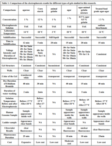
Electrophoresis was performed for human genome samples, and a ladder of agarose gel with TAE solution was used as a control for the studied samples: Corn starch gel with TAE solution, agarose gel with TAE solution, animal gelatin with TAE solution, agar with TAE solution, agar – animal gelatin mixture with TAE solution, and food grade agar-agar gelatin with a solution of sodium bicarbonate sodium hydroxide and sodium chloride. All experiments were carried out under similar conditions of pH and using the same equipment and tools. Many aspects were compared during the experiment on a repetitive level, and a mean of duration of solidification, texture, color, dye duration and other parameters are mentioned in Table1.
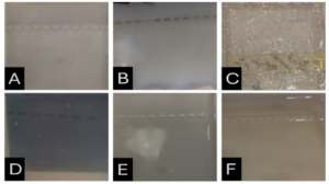
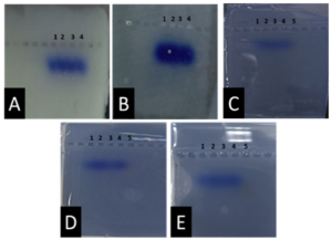
From Figure 1 we find that the animal gelatin gel (c) forms a surface ice layer and is not fully hardened. One of the reasons for this is the very low heat and low concentration of animal gelatin. Corn starch gel (B) gave a white color and similar properties in terms of the structure with agarose gel. Other gels gave properties in structure and color very similar to agarose gel.
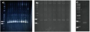
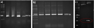
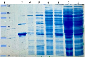
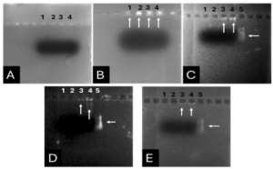
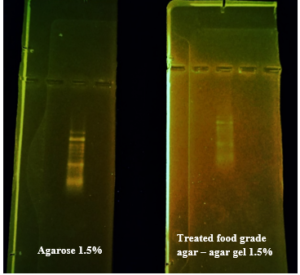
Before the samples were exposed to UV radiation, we can see from Figure 2 that the loading dye was electrophoresed for a distance of 1.2 cm in corn starch gel (A), for a distance of 1.7 cm in agar – gelatin mixture gel (B), for a distance of 0.9 cm for the loading dye and 1.3 cm for the Ladder in agar gel (C), for a distance of 1.4 cm for the loading dye and 1.7 cm for the Ladder in agarose gel (D), for a distance of 1.2 cm for the dye and 1.7 cm for the Ladder in treated food grade agar – agar gel (E) at the voltage and time shown in Table 1 for each gel mentioned. After the electrophoresis of 12% modified corn starch gel, 1% agar – animal gelatin mixture gel, 1% agar gel, 1% agarose gel, and 1.5 % of our treated food grade agar-agar gel with BS buffer, a separation of DNA was apparent, as shown in Figure 3, the modified Gel that is annotated with (E) in the Figure 3 shows good separation of the 50 bp DNA ladder (Vivantis®) in the 5th well, and the 4th well in E is genomic DNA extracted from human saliva. As for agarose gel D in Figure 3, good separation occurred in the 5th well and it showed resemblance to agarose gel in C. The gels were exposed to ultraviolet radiation and examined; we noticed that the disappearance of the fluorescence from the treated food grade agar-agar gel after 15 minutes, while the agarose retained its fluorescence for 25 minutes before the bands vanished from the UV. Knowing that the gels were dyed with the same type and concentration of dye and duration of time. For an electrophoresis buffer consisting of sodium bicarbonate, sodium hydroxide, and sodium chloride, it has shown high efficiency in securing the ions needed for electrophoresis while maintaining its physical and chemical properties; thus, it can be considered an equivalent solution to TAE solution. These results demonstrate the effectiveness of this variant using human genomic DNA. Electrophoresis with a ladder marker gave good results and good separation, as shown in Figure 4, which displays a comparison between agarose 1.5% and the treated food grade agar-agar gel 1.5%, where 5 µl of the marker was loaded into the wells in both gels at 40 V for 5 minutes and 80 V for 2 h followed by 30 minutes of soaking in an ethidium bromide tank. The results showed acceptable efficiency for the treated food-grade agar-agar similar to the efficiency of the agarose gel with some modifications in the method of work. Further enhancements of the images using gel documenting software could even make the separation look clearer for the treated food-grade agar -agar gel.
DISCUSSION
This research addressed finding a frugal alternative for agarose used in agarose gel DNA electrophoresis. The alternatives experimented in this research included: Agar, which originated in Japan in 1658. It was first introduced in the Far East and later in the rest of agarophyte seaweed-producing countries [29]. Agar is obtained from various genera and species of red–purple seaweeds—class Rhodophyceae—where it occurs as a structural carbohydrate in the cell walls and probably also plays a role in ion-exchange and dialysis processes [30]. Agar is a natural polymer commonly used in various fields of application, ranging from cosmetics to the food industry [31]. It is a gel forming polysaccharide with a main chain consisting of alternating 1,3-linked β-d-galactopyranose and 1,4-linked 3,6 anhydro-α-l-galactopyranose units [32]. Agarobiose is the basic disaccharide structural unit of all agar polysaccharides. Agar can be fractionated into two components: agarose and agaropectin [33]. The food-grade agar results were similar to agar results, yet microbiological agar can be more costly compared to food-grade agar-agar, and the treatment of agar with different salts described in this method gave slightly better results from previous research [12]. We also tested Starch, which is a major food source for humans. It is produced in seeds, rhizomes, roots, and tubers in the form of semi-crystalline granules with unique properties for each plant [34]. Edible and industrial corn starch was modified and used to prepare the electrophoresis gel. Corn starch is composed of two large α-linked glucose-containing polymers. Namely, smaller and nearly linear amylose and very large and highly branched amylopectin [35]. The starch alternative gel didn’t give good results and it was difficult to handle and too thick, so no DNA bands appeared [13]. Another alternative tested was Gelatin, which is a protein obtained by partial hydrolysis of collagen, which is the chief protein component in the skin, bones, hides, and white connective tissues of the animal body [36]. We can conclude from the gelatin gel result that it is not a good candidate for DNA gel electrophoresis, and this has been the case since the late 1980s.[11] From the results shown in Fig. 1, we can conclude that modifying the materials concentration allows us to control the structural and solidification properties. It is important to consider the appropriate gel concentration for the gel’s retinal structure, which is where electrophoresis samples pass, and this is in accordance with Bertasa et al. 2020 research that describes a stronger gel formation and crosslinks with increasing the concentration and anhydro units in the gel in addition to alterations of appearance and color, yet this didn’t apply to gelatin and starch where gelatin lacked the strength to solidify and the starch was too thick and difficult to handle after pouring because it solidified very quickly. [37] We can observe that the previously mentioned gels in Fig. 2 resulted in the electrophoresis of dyes at least, and this is logical because these gels create a charge neutral trap for the negatively charged loading dye to pass through in the presence of an electric field and an electrolyte. [38] From our results shown in Table 1, treated food grade agar-agar gel prepared with sodium bicarbonate solution was the most closely related alternative to the commonly used agarose gel with modifications in the working method to achieve very close results with agarose, while starch gel failed to give a proper result. Also, the mixture didn’t give a clear result because the DNA samples couldn’t get out of the wells. Agar gel, the same as agar – agar gel, gave results similar to those of agarose. But still, treated agar – agar gel showed better results than agar gel by the distance crossed by the DNA samples and the display of the samples, in addition to the low cost. This result of genomic DNA electrophoresis is well known and is confirmed by several previous researches, such as Green et al. 2019, where large genomic DNA fragments migrate slower than smaller fragments, and smearing marks in the resulting gel image refer to poor-quality DNA or electrophoresis conditions. [39] As for cost, 1 g of agarose costs around 35,000 Syrian pounds, while 1 g of agarose costs almost 2000 Syrian pounds, while 1 L of TBE 1x costs nearly 700,000 Syrian pounds, while SB buffer roughly costs 3500 Syrian pounds for the same amount, this makes this alternative 15 times cheaper than agarose gel, and 200 times cheaper for the electrolyte used. It seems from Fig. 4 that the treated food grade agar-agar can show strong bands from the ladder, and the separation requires more time; hence, it could be recommended to use it for PCR products of one band and a ladder with several strong bands, and the background fluorescence from ethidium bromide on the treated gel could mean that there should be more rinsing time for it, in order to give clearer bands.
Conclusions and Recommendations
This study offers a very low-cost alternative to agarose gel to help laboratories with limited income. We found that treated food grade agar-agar could give similar results to those of agarose gel, and by using other buffers for electrolyte like SB buffer. Based on the results of this study, this method provides a low-cost alternative to agarose and TBE & TAE, and it can be used by low-budget labs with limited budgets to make DNA assays more domesticated, where the alternatives suggested here cost 15 times less than the industrial agarose and electrolytes. Further research is recommended to enhance the clarity of the gel and explore the potential applications of this new gel in RNA separation and plasmid DNA separation and PCR amplicons of different lengths.